1 The Power Grid

This chapter outlines the legacy power grid: the infrastructure, sometimes described as the “world’s largest machine”, that delivers electrical power from generators to consumers using a complex hierarchy of interconnecting links. We start with basic electrical terms, then consider each major component of the grid in turn: generators, loads, and the network that interconnects them. We then discuss how these components interact when power flows along them during grid operation to continuously balance supply and demand and to match consumer payments with grid costs using an electricity market. Finally, we outline how the grid is monitored and controlled.

Prerequisites

Mathematics: Algebra, trigonometry, complex numbers, differential calculus, partial differentiation, systems of equations, Newton-Raphson method for numerical computation.
Physics: Basic understanding of electricity: current, voltage, resistance, inductance, and capacitance.

1.1 Basics

1.1.1 Currents and Circuits

The foundation of the power grid is the flow of electrons–a current–along an electrical conductor, usually a long metal wire, that forms an electrical circuit connecting the two terminals of a source of electrical energy such as a battery or a generator. These terminals are usually marked positive and negative. A current flows due to the difference in electric potential energy between these terminals (see Figure 1.1). The amount of work needed to move a unit charge (measured in Coulombs) from one terminal to another, or, more generally, between any two points in the circuit, is measured in Volts (V).

An analogy may be helpful. Consider two water containers connected by a pipe. If one container is raised above the other, then a current of water flows, due to the difference in gravitational potential energy, from the higher container to the lower.

1.1.2 Resistance

The rate of flow of an electrical current is proportional to the potential difference between the two end points of the circuit and inversely proportional to the degree to which the conductor resists the flow, a factor named resistance. Resistance is analogous to friction in the water pipe, which impedes the flow of water. If the potential difference between two points in the circuit is V Volts and the rate of flow is I Amperes, the resistance R is defined as $R = \frac{V}{I}$ Ohms (this is Ohm’s Law). A resistance of 1 Ohm means that a potential difference of 1 Volt will cause a current of 1 Ampere to flow. (This is a very low resistance! Typical resistances are in the range of kilo-Ohms to mega-Ohms.)

Resistance can be created using a device called a resistor which is depicted using this symbol:

Here is an example of a simple electrical circuit consisting of a voltage source (battery) connected to a resistor (Figure 1.1):

Figure 1.1: A simple electrical circuit consisting of a voltage source (battery) connected to a resistor. Current I flows from the positive terminal through the resistor to the negative terminal, driven by voltage V.

Resistance causes electrical energy to be converted into heat energy as the current flows through the conductor or resistor. This is known as Joule heating or resistive heating. The power dissipated as heat in a resistor can be calculated using the formula $P = I^2 R$, where P is the power lost in Watts, I is the current in Amperes, and R is the resistance in Ohms.

Resistance depends on the material, length, and cross-sectional area of the conductor. Materials with low resistivity, such as copper and aluminum, are commonly used for electrical wiring due to their low resistance. For a given material, resistance increases with length and decreases with cross-sectional area, following the formula $R = \rho \frac{L}{A}$, where $\rho$ is the resistivity of the material, L is the length, and A is the cross-sectional area. So, thicker and shorter wires have lower resistance.

To reduce losses, long distance power lines, which carry huge currents, are made of thick cables. Similarly, electric vehicles, which are charged using high currents, use noticeably thick cables for charging.

Example 1.1 Consider a conductor carrying a current of 10 Amperes with a resistance of 2 Ohms. The power dissipated as heat in the conductor can be calculated as follows:

$P = I^2 R = (10 \, \text{A})^2 \times 2 \, \Omega = 200 \, \text{Watts}$.

To reduce this power loss, we can increase the conductor thickness. By doubling the diameter, and hence the cross-sectional area of the conductor by a factor of 4, the resistance is reduced to 0.5 Ohms. The new power dissipation can be calculated as:

$P = I^2 R = (10 \, \text{A})^2 \times 0.5 \, \Omega = 50 \, \text{Watts}$.

Note that the power loss has been reduced by a factor of 4, but this also requires four times the material and can be expensive!

The resistance of a conductor also varies with temperature. For most conductive materials, resistance increases with temperature due to increased atomic vibrations that impede the flow of electrons. This relationship is often approximated linearly for small temperature ranges using the formula $R_T = R_0 [1 + \alpha (T - T_0)]$, where $R_T$ is the resistance at temperature $T$, $R_0$ is the resistance at a reference temperature $T_0$, and $\alpha$ is the temperature coefficient of resistance for the material.

Two resistors can be combined in two fundamental ways: in series or in parallel. When resistors are connected in series, the total resistance is the sum of the individual resistances: $R_{total} = R_1 + R_2 + ... + R_n$. When resistors are connected in parallel, the total resistance is given by the reciprocal of the sum of the reciprocals of the individual resistances: $\frac{1}{R_{total}} = \frac{1}{R_1} + \frac{1}{R_2} + ... + \frac{1}{R_n}$.

1.1.3 Power and Energy

A current flowing through a conductor transfers power to a load, which consumes this power to carry out some desirable activity. Power is measured in Watts (W). The power P delivered to a load by a voltage source is given by $P = VI$, where V is the voltage in Volts and I is the current in Amperes.

As a current flows over a conductor for a period of time, this results in the transfer of energy from the generator to the load. The total energy E, measured in Joules (J), transferred over a time period t (in seconds) is given by $E = Pt = VIt$. Thus, power is the instantaneous rate of energy transfer, and can also be measured in Joules per second (1 Watt = 1 Joule/second).

Continuing our analogy, power can be thought of rate at which water flows through the pipe, while energy is the total amount of water that has flowed over a certain period of time. From a computer science perspective, power is analogous to the rate of information transfered, measured in bits/second and energy is analogous to the total amount of data transferred in bits

When transferring large amounts of power, rather than using thick conductors, power transmission systems aim to minimize current flow by using high voltages, which allows for efficient power delivery with lower losses. By increasing voltage and reducing current, power can be transmitted more efficiently over long distances. We will return to this topic in the section on power transmission.

Example 1.2 Suppose you want to transfer power at the rate of 100 W for 10 seconds, resulting in a transfer of 1,000 Joules of energy. This can be done in multiple ways. For example, we could use a voltage of 10 Volts or 100 Volts. Suppose we use a voltage of 10 Volts and the current is carried on a conductor with some resistance R. Then, the required current can be calculated as

$I = \frac{P}{V} = \frac{100 \, \text{W}}{10 \, \text{V}} = 10 \, \text{A}$ resulting in heating loss $P_{loss} = I^2 R = (10 \text{A})^2 \times R = 100R$ Watts.

By increasing the voltage to 100 Volts, the required current decreases to

$I = \frac{P}{V} = \frac{100 \, \text{W}}{100 \, \text{V}} = 1 \, \text{A}$, resulting in a heating loss $P_{loss} = I^2 R = (1 \, \text{A})^2 \times R = 1R$ Watts, a reduction by a factor of 100.

This demonstrates that increasing the voltage leads to a significant reduction in resistive losses.

1.1.4 Kirchhoff’s Laws

In any electrical circuit, two fundamental laws govern the behavior of currents and voltages: Kirchhoff’s Current Law (KCL) and Kirchhoff’s Voltage Law (KVL).

Kirchhoff’s Current Law (KCL) states that the total current entering a junction (or node) in an electrical circuit must equal the total current leaving that junction. This is based on the principle of conservation of electric charge, which implies that charge cannot accumulate at a node. Mathematically, KCL can be expressed as:
\[\sum I_{in} = \sum I_{out}\]

where $I_{in}$ is the current entering the node and $I_{out}$ is the current leaving the node.

Kirchhoff’s Voltage Law (KVL) states that the sum of the electrical potential differences (voltages) around any closed loop in a circuit must equal zero. This is based on the principle of conservation of energy, which implies that the total energy gained by charges as they move through voltage sources must equal the total energy lost as they move through resistive elements and other components in the loop. Mathematically, KVL can be expressed as:
\[\sum V = 0\]

where $V$ represents the voltage drops and rises around the closed loop.

Example 1.3 Consider a simple circuit with a 12V battery connected to three resistors: $R_1 = 2\, \Omega$, $R_2 = 3\, \Omega$, and $R_3 = 1\, \Omega$. The resistors $R_1$ and $R_2$ are connected in series, and their combination is in parallel with $R_3$.

Figure 1.2: Circuit diagram illustrating Kirchhoff’s Laws. A 12V battery is connected to resistors R₁ (2Ω) and R₂ (3Ω) in series, with R₃ (1Ω) in parallel. Current I_total splits at node A into I₁ (through R₁ and R₂) and I₂ (through R₃).

Applying Kirchhoff’s Current Law (KCL):

At the junction where the current splits to flow through $R_3$ or through the series combination of $R_1$ and $R_2$, KCL tells us:

\[I_{total} = I_1 + I_2\]

where $I_{total}$ is the current from the battery, $I_1$ is the current through $R_1$ and $R_2$ (same current flows through both since they’re in series), and $I_2$ is the current through $R_3$.

Applying Kirchhoff’s Voltage Law (KVL):

For the loop containing the battery and the series combination $R_1$ and $R_2$:

\[V_{battery} - I_1 R_1 - I_1 R_2 = 0\] \[12\, \text{V} - I_1(2 + 3)\, \Omega = 0\] \[I_1 = \frac{12}{5} = 2.4\, \text{A}\]

For the loop containing the battery and $R_3$:

\[V_{battery} - I_2 R_3 = 0\] \[12\, \text{V} - I_2(1)\, \Omega = 0\] \[I_2 = 12\, \text{A}\]

Using KCL: $I_{total} = 2.4 + 12 = 14.4\, \text{A}$

This example shows how KCL ensures current conservation at junctions, while KVL ensures energy conservation around closed loops.

Note that the power dissipated in the left hand branch is given by $P_1 = I_1^2 (R_1 + R_2) = (2.4 \, \text{A})^2 \times 5 \, \Omega = 28.8 \, \text{W}$, and in the right hand branch by $P_2 = I_2^2 R_3 = (12 \, \text{A})^2 \times 1 \, \Omega = 144 \, \text{W}$. The total power supplied by the battery is $P_{total} = V_{battery} \times I_{total} = 12 \, \text{V} \times 14.4 \, \text{A} = 172.8 \, \text{W}$, which equals the sum of the power dissipated in both branches: $P_1 + P_2 = 28.8 \, \text{W} + 144 \, \text{W} = 172.8 \, \text{W}$, confirming energy conservation.

What would happen if we added another resistor in series with $R_3$? How would that affect the currents and voltages in the circuit? Try analyzing it using KCL and KVL!

1.1.5 Voltage and Current Sources

In electrical circuits, two fundamental types of sources are used to provide energy: voltage sources and current sources.
A voltage source maintains a fixed voltage across its terminals regardless of the current flowing through it. A current source, on the other hand, maintains a fixed current through its terminals regardless of the voltage across it. These sources are idealized components used in circuit analysis to model real-world power supplies and loads.

1.1.6 Alternating Current

Thus far, we have made the implicit assumption that the current flows only in one direction, from the positive terminal of the source to its negative terminal. This type of current is called direct current (DC). However, in most power grids, the current alternates direction periodically; this is called alternating current (AC). This is like the water containers being alternately raised and lowered, causing the water to flow back and forth in the connecting pipe. We will see later why AC is used in power grids (it has to do with the ease of transforming voltages using transformers).

The frequency of this alternation is typically 50 or 60 alternations or cycles per second, also denoted Hertz abbreviated Hz. In an AC circuit, the voltage and current amplitudes alternate sinusoidally between positive and negative values, with periodic zero crossings, when the flow of current is momentarily zero.

Figure 1.3: Sinusoidal variation of voltage and current over time in an AC circuit. The voltage (solid blue line) and current (dashed red line) both vary sinusoidally with time, completing one full cycle in period T. For a purely resistive load, voltage and current are in phase.

1.1.6.1 Complex Numbers for AC Analysis

Before we dive into AC circuit analysis, we need a mathematical tool: complex numbers.

A complex number is a tuple or vector in 2D that has two parts: a real part and an imaginary part. We write it as $z = a + jb$, where $a$ is the real part, $b$ is the imaginary part, and $j = \sqrt{-1}$ (engineers use $j$ instead of $i$ to avoid confusion with current $I$).

Complex numbers add like vectors, with the real and complex parts added separately. In the complex plane, this forms a parallelogram, and the diagonal is the sum. They have two equivalent representations:

Rectangular: $z = a + jb$ (easy for addition/subtraction)
Polar: $z = r\angle\theta$ (easy for multiplication/division)
Polar → Rectangular: $a = r\cos(\theta)$, $b = r\sin(\theta)$
Rectangular → Polar: $r = \sqrt{a^2 + b^2}$, $\theta = \arctan(b/a)$

The interactive example here should help you get some intuition about complex numbers.

1.1.6.2 Phasors

It is often useful to represent the sinusoidal voltage and current in an AC circuit using phasors, which are rotating vectors in the complex plane. We can think of the tip of the phasor as tracing out a circle in the complex plane as it rotates, with the projection onto the real (X) axis giving the instantaneous voltage or current value at any point in time. The length of the phasor represents the amplitude of the voltage or current, while the angle of the phasor represents the phase of the waveform relative to a reference point in time. The rate of change of the phasor angle corresponds to the frequency of the AC signal.

The voltage phasor is represented as $V = V_0 e^{j\omega t}$¹, where $V_0$ is the amplitude, $\omega$ is the angular frequency (related to frequency $f$ by $\omega = 2\pi f$), and $t$ is time. The current phasor is represented similarly as $I = I_0 e^{j(\omega t + \phi)}$, where $I_0$ is the current amplitude and $\phi$ is the phase angle between voltage and current.

The animation below illustrates this concept, showing how a rotating phasor on the left generates a sinusoidal waveform on the right:

Figure 1.4: Animation showing the relationship between a rotating phasor and its sinusoidal waveform. The phasor rotates counterclockwise in the complex plane (left), and its projection onto the real axis (shown by the red dashed line) creates the cosine wave (right). Use the Start button to start the animation.

Kirchhoff’s Voltage Law (KVL) and Kirchhoff’s Current Law (KCL) still apply in AC circuits, but we must account for the complex nature of voltages and currents due to phase differences. When applying KVL, the sum of the complex voltages around any closed loop must equal zero, taking into account both magnitude and phase. Similarly, KCL states that the sum of complex currents entering a node must equal the sum of complex currents leaving that node—this is exactly analogous to flow conservation constraints in network flow algorithms, where the total flow into a node equals the total flow out (except at source and sink nodes).

A voltage phasor is represented as $V = 120\angle 30°$ V. What are its real and imaginary components in rectangular form?
True or False: If two AC voltages have the same magnitude but different phase angles, they represent the same physical voltage at any instant in time.
In phasor representation, what physical quantity does the angle of a phasor represent?

Can’t answer confidently? Review Complex Numbers for AC Analysis.

1.1.7 Capacitors and Inductors

A capacitor is a device that stores energy in the form of an electric field, like a rubber membrane replacing part of a water pipe, which stores water when filled and releases it when needed, helping to smooth out fluctuations in water flow. It typically consists of two conductive plates or surfaces separated by an insulating material (called the dielectric). When a voltage is applied across the plates, an electric field develops, causing positive charge to accumulate on one plate and negative charge on the other. Because of this, capacitors resist changes in current flow.

Capacitors are characterized by their capacitance, measured in Farads (F) and are depicted using this symbol:

An inductor is a device that stores energy in the form of a magnetic field, where the field is self-induced by the flow of current. It typically consists of a coil of wire. When current flows through the coil, it generates a magnetic field around it, which then impedes the flow of current. The voltage across an inductor is proportional to the rate at which the current is changing. Inductors are characterized by their inductance, measured in Henrys (H) and are depicted using this symbol:

When placed in a DC circuit, capacitors eventually block current flow after being fully charged, while inductors allow steady current to flow after an initial surge. However, in AC circuits, both capacitors and inductors continuously influence the flow of current due to the changing voltage and current levels.

Preview: Phase Relationships

In the next section, we’ll describe HOW capacitors and inductors affect AC currents—specifically, they create phase shifts between voltage and current. The detailed mathematical WHY requires understanding reactance and impedance, which we’ll cover in Section 1.1.8.

If the phase relationships feel mysterious at first, that’s expected! We’ll build physical intuition now, then return with full mathematical derivations later. Think of this as a preview of a key phenomenon you’ll fully understand by the end of this chapter.

1.1.7.1 Phase Relationships

In AC circuits, capacitors and inductors cause the voltage and current to be out of phase with each other. Specifically, in a circuit with an ideal capacitor, the current leads the voltage by 90 degrees, while in a circuit with an ideal inductor, the voltage leads the current by 90 degrees.

Why does current lead voltage in a capacitor?

Recall that a capacitor is like a rubber membrane in a pipe - you must push water (current) against it before it stretches (voltage builds up). In the same way, to change the voltage across a capacitor, you must first move charge onto its plates. This means current must flow before voltage can change.

Here’s the intuitive sequence in an AC circuit with an ideal capacitor:

When supply voltage is at zero and starting to increase (go positive), charge rushes onto the plates
This creates a large current flow right when voltage is zero. So current is at its peak when voltage is zero.
As charge accumulates, voltage across the capacitor builds up
When the plates are fully charged, the supply current has come to a stop (is zero) but the voltage across the plates reaches its maximum, so that the outflow of charge is at its peak.
A similar sequence happens when voltage goes negative. The charge flows off the plates the fastest when the voltage is zero, and the voltage reaches its negative peak when the current is zero.
Therefore, the current reaches its peak before the voltage does → current leads voltage

Why does voltage lead current in an inductor?

The voltage across an inductor is proportional to its inductance as well as the rate of change of current, with the fundamental relationship being $V = L \frac{dI}{dt}$. This means the voltage measured across an inductor is proportional to how quickly the current is changing, not the current itself.

Here’s the intuitive sequence of actions in an AC circuit with an ideal inductor:

When current is at zero and starting to increase, it’s changing most rapidly
This rapid change in current creates a maximum voltage across the inductor (trying to oppose the change)
When current reaches its maximum value, it momentarily stops changing ($\frac{dI}{dt} = 0$). At this instant, voltage across the inductor is zero
Therefore, the voltage reaches its peak before the current does → voltage leads current
A similar sequence happens when current goes negative. When the current is changing most rapidly (crossing zero), voltage is at its peak, and when current is at its negative peak, voltage is zero.

1.1.7.2 Phasor Representation

Phasors provide a convenient way to visualize phase relationships in AC circuits. The figure below shows phasor diagrams showing the voltage and current phasors for capacitive and inductive circuits:

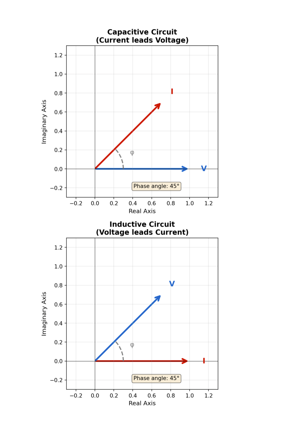
Figure 1.5: Phasor diagrams showing phase relationships. Top: Capacitive circuit where current (I) leads voltage (V) by angle φ. Bottom: Inductive circuit where voltage (V) leads current (I) by angle φ. The phasors rotate counterclockwise, and their projection onto the vertical axis gives the instantaneous values.

The interactive visualizations below demonstrate these phase relationships. You can adjust the capacitance and inductance values to see how they affect the phase shift between voltage and current. Notice that the current leads voltage in the capacitor circuit and voltage leads current in the inductor circuit. Also, observe how increasing capacitance decreases the phase angle in the capacitor circuit, while increasing inductance increases the phase angle in the inductor circuit.

Because of the phase differences introduced by capacitors and inductors, not all the power supplied by the source is dissipated as heat in resistive elements. Some of it is temporarily stored in the electric and magnetic fields of capacitors and inductors, respectively, and then returned to the source. This leads us to the concepts of reactance and impedance.

1.1.8 Reactance

In AC circuits, capacitors and inductors introduce additional resistance to current flow, known as reactance. Reactance is measured in Ohms (Ω), similar to resistance, and is the frequency-dependent resistance that affects how much current flows in response to an applied AC voltage. The higher the reactance, the lower the current for a given voltage, similar to resistance in DC circuits. Reactance does not appear in a DC circuit and can therefore be thought of as the penalty paid for using AC.

Capacitive reactance ($X_C$), defined as $X_C = \frac{1}{2\pi fC}$ where $f$ is the AC frequency and $C$ is the capacitance, decreases with increasing values of both capacitance and frequency, while inductive reactance ($X_L$) defined as $X_L = 2 \pi f L$, where $L$ is the inductance, increases with both inductance and frequency. The total reactance ($X$) in a circuit containing both capacitive and inductive elements is given by $X = X_L - X_C$. If $X$ is positive, the circuit is said to be inductive (inductive reactance dominates), while if $X$ is negative, the circuit is capacitive (capacitive reactance dominates).

1.1.9 Impedance

So far we’ve learned that resistance opposes current and dissipates energy as heat, while reactance opposes current and stores energy in electric or magnetic fields. But in real AC circuits, every component has both resistance and reactance operating simultaneously—a motor has resistance in its copper windings (causing heating) and inductance from its magnetic field (storing energy), while a transmission line has resistive losses in the conductors and inductive/capacitive effects from the electromagnetic fields around the wires. The combined effect of resistance and reactance is called impedance ($Z$), which determines the overall opposition to current flow in an AC circuit.

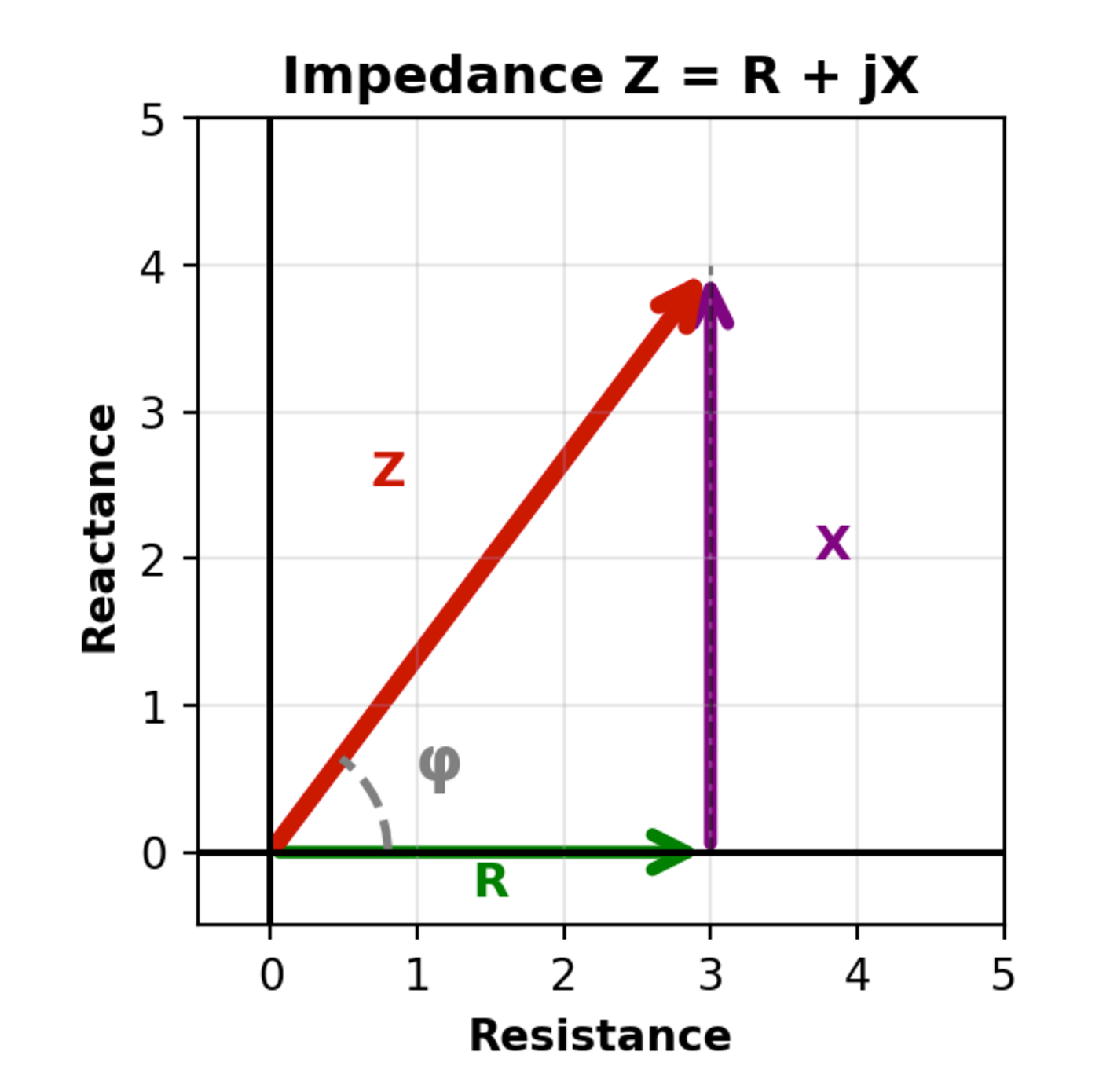
Impedance is a complex quantity, expressed as $Z = R + jX$, where $R$ is resistance, $X = X_L - X_C$ is reactance, and $j$ is the imaginary unit. The magnitude of impedance is given by $|Z| = \sqrt{R^2 + X^2}$, and the phase angle is $\phi = \tan^{-1}(\frac{X}{R})$.

Revisiting Phase Shifts: The Mathematical Explanation

Earlier in Section 1.1.7.1, we observed that current leads voltage in capacitors and lags in inductors. Now we can explain why mathematically:

The key insight: Reactance creates a 90° phase shift, represented by the imaginary unit $j$ in impedance.

Pure capacitor: $Z_C = -jX_C$ (purely imaginary, negative)
- The $-j$ term rotates the current phasor by -90° relative to voltage
- This means current leads voltage by 90°
Pure inductor: $Z_L = jX_L$ (purely imaginary, positive)
- The $+j$ term rotates the current phasor by +90° relative to voltage
- This means voltage leads current by 90° (or current lags voltage by 90°)

The $j$ operator in complex numbers performs a 90° rotation in the complex plane. This mathematical property perfectly captures the physical phenomenon of phase shifts in reactive components! When we write $Z = R + jX$, the imaginary part ($jX$) controls the phase relationship between voltage and current.

The diagram below illustrates how impedance is represented graphically as a vector in the complex plane, with resistance R on the real axis and reactance X on the imaginary axis:

Figure 1.6: Impedance triangle showing how impedance Z is computed from resistance R and reactance X. R lies on the real axis, X on the imaginary axis, and Z is the vector sum with magnitude |Z| and phase angle φ.

Comparison: Resistance, Reactance, and Impedance

Property	Resistance (R)	Reactance (X)	Impedance (Z)
What it represents	Opposition to current due to energy dissipation	Opposition to current due to energy storage	Total opposition to AC current
Energy behavior	Dissipates as heat (irreversible)	Stores and releases each cycle (reversible)	Combination of both
Formula	$R = \frac{V}{I}$ (Ohm’s law)	$X_C = \frac{1}{2\pi fC}$ (capacitor) $X_L = 2\pi fL$ (inductor)	$Z = R + jX$ $\|Z\| = \sqrt{R^2 + X^2}$
Units	Ohms (Ω)	Ohms (Ω)	Ohms (Ω)
DC behavior	Same value as AC (frequency-independent)	Capacitor: $X_C \to \infty$ (blocks current) Inductor: $X_L \to 0$ (acts like wire)	Reduces to pure resistance: $Z = R$
AC behavior	Independent of frequency	Frequency-dependent $X_C$ decreases as $f$ increases $X_L$ increases as $f$ increases	Frequency-dependent via reactance
Phase shift	0° (voltage and current in phase)	±90° Capacitor: current leads by 90° Inductor: voltage leads by 90°	$\phi = \arctan(\frac{X}{R})$ (between 0° and ±90°)
Mathematical representation	Real number	Imaginary number ($jX$)	Complex number ($R + jX$)
Power dissipation	Yes - converts to heat ($P = I^2R$)	No - energy oscillates	Resistive part dissipates, reactive part stores/releases
Example value	50 Ω resistor in light bulb	30 Ω inductive reactance in motor at 60 Hz	$50 + j30$ Ω Magnitude: 58.3 Ω Angle: 31°
Common applications	Heating elements, power dissipation, current limiting	Energy storage, filtering, power factor correction	Complete circuit analysis, power system modeling

Example 1.4 Problem: A transmission line has resistance $R = 3$ Ω and inductive reactance $X_L = 4$ Ω. Calculate:

The complex impedance $Z$
The impedance magnitude $|Z|$
The phase angle $\phi$
Interpret the results

Solution:

Since impedance is $Z = R + jX$: \[Z = 3 + j4 \text{ Ω}\]

Using the Pythagorean theorem: \[|Z| = \sqrt{R^2 + X^2} = \sqrt{3^2 + 4^2} = \sqrt{9 + 16} = \sqrt{25} = 5 \text{ Ω}\]

The phase angle \[\phi = \arctan\left(\frac{X}{R}\right) = \arctan\left(\frac{4}{3}\right) = 53.1°\]

We can also express impedance in polar form: $Z = 5\angle 53.1°$ Ω

The magnitude (5 Ω) represents the total opposition to current flow
The phase angle (53.1°) tells us the current will lag the voltage by 53.1° (inductive circuit)
Since $X > R$, the circuit is predominantly inductive (reactive component is larger than resistive)
If connected to a 120V AC source, the current would be: $I = V/|Z| = 120/5 = 24$ A RMS

The magnitude of impedance affects the amplitude of current flow. Specifically, Ohm’s Law for AC circuits is expressed as $V = IZ$, where $V$ and $I$ are the Root Mean Square (RMS) voltage and current, respectively, defined as the effective values of voltage and current over a cycle and given by $V_{RMS} = \frac{V_0}{\sqrt{2}}$ and $I_{RMS} = \frac{I_0}{\sqrt{2}}$ where $V_0$ and $I_0$ are the peak amplitudes, $R$ is the resistance, and $Z$ is the impedance. The root mean square (RMS) values are used because they provide a measure of the equivalent DC value that would deliver the same power to a resistive load. This is particularly useful in AC circuits where voltages and currents vary sinusoidally over time. They are computed by taking the square root of the average of the squares of the instantaneous values over one complete cycle, a simple integral defined as $V_{RMS} = \sqrt{\frac{1}{T} \int_0^T v(t)^2 dt}$ for voltage and similarly for current.

Example 1.5 Consider an AC circuit with a resistance of 3 Ω and an inductive reactance of 4 Ω connected to a 120 V (RMS) AC source at 60 Hz.

First, calculate the impedance magnitude:

$|Z| = \sqrt{R^2 + X_L^2} = \sqrt{3^2 + 4^2} = \sqrt{9 + 16} = 5 \, \Omega$

The phase angle between voltage and current is:

$\phi = \tan^{-1}\left(\frac{X_L}{R}\right) = \tan^{-1}\left(\frac{4}{3}\right) = 53.1°$

Using Ohm’s Law for AC circuits, the current (RMS) flowing through the circuit is:

$I = \frac{V}{|Z|} = \frac{120 \, \text{V}}{5 \, \Omega} = 24 \, \text{A (RMS)}$

Since this is an inductive circuit (positive reactance), the current lags the voltage by 53.1°. This means that when the voltage reaches its peak, the current is still climbing toward its peak, which it reaches 53.1° (or about 2.5 ms at 60 Hz) later.

If we wanted to calculate the peak current, we would use:

$I_0 = I_{RMS} \times \sqrt{2} = 24 \times 1.414 = 33.9 \, \text{A (peak)}$

A circuit element has impedance $Z = 6 + j8$ Ω. What is the magnitude $|Z|$ and phase angle $\phi$?
True or False: Impedance is frequency-dependent because the reactive component (X) changes with frequency, but the resistive component (R) remains constant.
If an inductor has reactance $X_L = 10$ Ω at 60 Hz, what happens to $X_L$ if the frequency increases to 120 Hz?

Can’t answer confidently? Review the Impedance section and the worked example above.

1.1.10 Conductance, Susceptance, and Admittance

These related concepts are useful when analyzing AC circuits, especially in power systems. Consider a circuit element between nodes $i$ and $j$ with impedance $Z_{ij} = R_{ij} + jX_{ij}$.

The admittance ($Y_{ij}$) represents how easily current can flow through a circuit and is defined as the reciprocal of the impedance. That is, $Y_{ij} = G_{ij} + jB_{ij} =\frac{1}{Z_{ij}} = \frac{1}{R_{ij} + jX_{ij}} = \frac{R_{ij} - jX_{ij}}{R_{ij}^2 + X_{ij}^2}$. The magnitude of admittance is given by $|Y| = \sqrt{G^2 + B^2}$, and the phase angle is $\theta = \tan^{-1}(\frac{B}{G})$.
The conductance ($G_{ij}$) is the real part of admittance and is given by $= \frac{R_{ij}}{R_{ij}^2 + X_{ij}^2}$. $G$ is measured in Siemens (S) or mhos (℧).
The susceptance ($B_{ij}$) $ = -$ is the imaginary part of the admittance.

Figure 1.7: Relationships between impedance, resistance, reactance, admittance, conductance, and susceptance in AC circuits. The diagram shows how these quantities are related through reciprocals and complex number representations.

Here is an example of how to calculate admittance:

Example 1.6 Consider an AC circuit with a resistance of 4 Ω and a capacitive reactance of 3 Ω. First, calculate the impedance: $Z = R + jX = 4 - j3 \, \Omega$ (-j3 not j3 because this is capacitive).
Then, calculate the admittance:
$Y = \frac{1}{Z} = \frac{1}{4 - j3} = \frac{4 + j3}{(4)^2 + (-3)^2} = \frac{4 + j3}{16 + 9} = \frac{4 + j3}{25} = 0.16 + j0.12 \, S$. We can now identify the conductance and susceptance:

Conductance: $G = 0.16 \, S$
Susceptance: $B = 0.12 \, S$

1.1.11 Real and Reactive Power, and the Power Factor

In AC circuits, unlike DC circuits, phase differences between voltage and current caused by reactive components (capacitors and inductors) consume power. These components both store and release energy, leading to power loss that does not perform any net work over a complete cycle. Even though reactive power doesn’t do useful work, it requires real current to flow through wires, transformers, and generators. This current causes $I^2R$ losses and requires higher equipment ratings.

Consider a motor connected to the power grid: it draws current from the grid not only to do mechanical work (turning a shaft) but also to maintain its magnetic fields. This magnetic field energy moves back and forth between the motor and the power source twice per AC cycle—it doesn’t do any useful work, but the current carrying this energy still flows through transmission lines, causing resistive losses and requiring thicker conductors.

How do we account for power that “flows” but doesn’t get consumed? And how do we distinguish between power that does useful work versus power that merely sustains electromagnetic fields?

The answer lies in decomposing power into multiple components: real power (measured in watts) that actually performs work and generates heat, reactive power (measured in volt-amperes reactive, or VARs) that sustains electromagnetic fields, and apparent power (measured in volt-amperes, or VA) that represents the total power flow the grid infrastructure must support. Understanding these distinctions is essential for power system design, equipment sizing, and grid operation.

First, let us consider a purely resistive AC circuit where voltage and current are in phase. In such a system, all the power supplied by the source is dissipated as heat in the resistive elements and is given by the same formula as in DC circuits, $P = I_{rms}^2 R$ or $P = \frac{V_{rms}^2}{R}$, where $I_{rms}$ and $V_{rms}$ are the root mean square (RMS) values of current and voltage, respectively and computed as $V_{rms} = \frac{V_0}{\sqrt{2}}$ and $I_{rms} = \frac{I_0}{\sqrt{2}}$.

Now, suppose that the AC circuit has inductive or capacitive elements. In this circuit, there will be a phase difference between voltage and current. Then, the average power dissipated by the circuit is reduced (because it does less work). Specifically, the average power is given by $P = V_{rms} I_{rms} \cos(\phi)$, where $\phi$ is the phase angle between voltage and current.

We define the three types of power in AC circuits:

Real power (measured in Watts, W) is the actual power consumed by resistive components and converted into useful work or heat. This is the power that does something useful—it lights bulbs, turns motors, and heats water.
Reactive power (measured in Volt-Amperes Reactive, VAR) is the power that oscillates back and forth between the source and reactive components (capacitors and inductors). It’s not consumed but rather borrowed and returned twice per cycle. Imagine pushing a child on a swing—you need to supply energy to keep the swing going, but the swing returns that energy back to you on each cycle. Reactive power is necessary to maintain electric and magnetic fields in motors, transformers, and other inductive/capacitive devices, but it doesn’t perform any net work. This is the “wasted” power that doesn’t do useful work but is essential for the operation of AC systems.
Apparent power (measured in Volt-Amperes, VA) is the product of RMS voltage and current, representing the total power that appears to flow in the circuit. It’s the vector sum of real and reactive power, given by $S = \sqrt{P^2 + Q^2}$, where $P$ is real power and $Q$ is reactive power. Apparent power represents the capacity that the power system must provide, even though not all of it does useful work. This is why generators and transformers are rated in VA rather than Watts—they must handle the total current flowing through them, regardless of whether that current is doing useful work or just sloshing back and forth.

The power factor (PF) of an AC circuit is defined as the cosine of the phase angle between voltage and current, i.e., $PF = \cos(\phi)$. A power factor of 1 indicates that voltage and current are in phase, meaning all the power supplied by the source is being used effectively (the ideal situation). A power factor less than 1 indicates that some power is being stored and released by reactive components (capacitors and inductors), leading to inefficiencies in power delivery. A leading power factor (current leads voltage) indicates a capacitive load, while a lagging power factor (current lags voltage) indicates an inductive load.

A system with a lower power factor requires a higher current for the same amount of useful power delivered, leading to increased losses in the power system, because these are proportional to the square of the current). In power systems, maintaining a high power factor is crucial for efficient operation, as it reduces losses in transmission lines and improves voltage regulation. The power factor can be corrected using capacitors or inductors to counteract the effects of inductive or capacitive loads, respectively. In practical power systems, loads, such as motors, are often inductive, resulting in a lagging power factor and this can be corrected using a capacitor bank. The power factor is usually close to 1 in well-designed systems and not something that is typically calculated in basic power grid analysis.

Comparison: Real, Reactive, and Apparent Power

Property	Real Power (P)	Reactive Power (Q)	Apparent Power (S)
What it represents	Power that does useful work	Power that oscillates between source and load	Total power capacity required
Formula	$P = VI\cos(\phi)$	$Q = VI\sin(\phi)$	$S = VI$ $S = \sqrt{P^2 + Q^2}$
Units	Watts (W) kilowatts (kW) megawatts (MW)	Volt-Ampere Reactive (VAR) kiloVAR (kVAR) megaVAR (MVAR)	Volt-Ampere (VA) kiloVA (kVA) megaVA (MVA)
Physical meaning	Energy converted to heat, light, motion, etc. (irreversible)	Energy stored in electric/magnetic fields, returned each cycle (reversible)	Vector sum of real and reactive power
Direction of flow	One-way: source → load	Two-way: oscillates back and forth	N/A (not a flow, but a capacity)
DC circuits	$P = VI$ (the only type of power)	Zero (no oscillation in DC)	Same as real power: $S = P$
AC circuits (resistive load)	$P = VI$ when $\phi = 0°$	Zero when $\phi = 0°$	Same as real power when resistive
AC circuits (reactive load)	$P < S$ when $\phi \neq 0°$	Maximum when $\phi = 90°$ (pure reactance)	Always $S \geq P$
What limits generators?	Not the primary constraint	Not the primary constraint	This is the limiting factor - generators rated in MVA
Example	800 kW electric heating	600 kVAR inductive motor load	1000 kVA transformer capacity

1.1.12 Transformers

We have seen that higher voltages lead to lower currents and thus lower losses in power transmission. However, most electrical devices operate at much lower voltages. To efficiently transmit power over long distances and then step it down to usable levels, we use transformers. A transformer is a static electrical device that transfers electrical energy between two or more circuits through electromagnetic induction. Transformers consist of two or more coils of wire (called windings) wrapped around a common core consisting of a magnetic material. When an alternating current flows through the primary winding, it creates a changing magnetic field that induces a voltage in the secondary winding. The ratio of the number of turns in the primary winding to the number of turns in the secondary winding determines whether the transformer steps up (increases) or steps down (decreases) the voltage.

Figure 1.8: Schematic diagram of a transformer showing primary and secondary windings around an iron core. The transformer converts voltage levels while maintaining power (neglecting losses).

In this example, the transformer has a turns ratio of $N_P/N_S = 8/4 = 2$, making it a step-down transformer that reduces voltage by half (if $V_P = 240$ V, then $V_S = 120$ V). Conversely, the current increases by a factor of 2 to conserve power: if $I_P = 10$ A, then $I_S = 20$ A.

Transformers are highly efficient, often exceeding 95% efficiency, meaning that very little power is lost during the voltage transformation process. However, real transformers do have some losses due to factors such as winding resistance (copper losses) and core hysteresis and eddy currents (iron losses). These losses are typically small but important to consider in large-scale power systems.

Transformers allow us to transmit electrical power at high voltages (and low currents) over long distances, minimizing losses, and then step down the voltage to safer, usable levels for homes and businesses. That is one reason why the power grid mainly uses AC rather than DC for transmission (although modern advancements in power electronics are making high-voltage DC transmission more feasible for certain applications). Another reason is that power systems actually transmit power in three phases, which we cover next.

1.1.13 Three-Phase Power Systems

A key innovation in power systems is the use of three-phase power for generation, transmission, and distribution. In a three-phase system, three separate AC voltages are generated and transmitted, each offset by 120 degrees in phase. We can represent this by three voltage and current phasors that are offset 120 degrees from each other, as shown below:

Figure 1.9: Three-phase voltage phasor diagram showing three voltage phasors (Va, Vb, Vc), each separated by 120 degrees. The phasors rotate counterclockwise at the same angular frequency. Current phasors are similarly offset by 120 degrees. The three phasors sum to zero at any instant in a balanced system.

This configuration provides several advantages over single-phase power:
* It delivers a more constant power transfer to loads, reducing pulsations and improving efficiency.
* It allows for smaller and more efficient wiring and transformers, as the total power is split across three conductors. * It enables the use of three-phase motors, which are more efficient and have better starting torque than single-phase motors.
* It provides redundancy; if one phase fails, the system can often continue to operate at reduced capacity.

Amazingly, three-phase power can be transmitted using only three wires (one for each phase) making it more economical for long-distance transmission and distribution! This is because the sum of the instantaneous voltages in a balanced three-phase system is always zero, allowing for a neutral conductor to be omitted or using the Earth itself as a return path, since soil contains ions that can conduct electricity. This is a neat trick, in that it dramatically reduces the amount of conductor material needed for power transmission and was one of the key innovations that enabled the widespread adoption of AC power systems. The invention of the three-phase system is credited to Nikola Tesla in the late 19th century and it enabled Westinghouse to build the first large-scale AC power systems, which ultimately won out over Edison’s DC systems in the “War of Currents”.

While the power grid uses three-phase power for transmission and distribution, most homes receive only single-phase power. When you look at your home’s electrical panel, you’ll typically see wiring with three types of conductors:

Hot wire (usually black or red): This carries one phase of the AC voltage, typically 120V in North America (230V in Europe/Asia) relative to ground. In homes with 240V service, there are actually two hot wires carrying opposite phases (180° apart), which when combined provide 240V for large appliances like electric dryers and ovens.
Neutral wire (usually white): This provides the return path for current and is connected to ground at the service panel. The voltage between hot and neutral is the standard household voltage (120V or 230V depending on the country).
Ground wire (usually green or bare copper): This is a safety conductor connected to the Earth (literally buried in the ground via a grounding rod or water pipe). It doesn’t carry current during normal operation but provides a safe path for fault currents, protecting you from electric shock if a wire becomes loose and touches a metal appliance case.

The power company taps into one of the three phases from the distribution transformer on your street to provide power to your home. Your neighbors might be connected to different phases to balance the load across all three phases in the neighborhood. This is why a power outage might affect only some houses on your street—if one phase fails, only the homes connected to that phase lose power!

Key Concepts Review

Now is a good time to check your understanding of these fundamental electrical concepts:

Voltage, current, resistance, and power
Ohm’s Law as applied to both DC and AC circuits
Alternating current (AC), frequency, and sinusoidal waveforms
Phasors and their representation in the complex plane
Capacitors and inductors and their behavior in AC circuits
Phase relationships between voltage and current
Reactance (capacitive and inductive) and impedance
Real power, reactive power, and apparent power
Power factor and its significance in AC circuits
Transformers and voltage transformation
Three-phase power systems and their advantages

1.2 Grid Elements

1.2.1 Overview

Much like a simple circuit (Figure 1.1), the power grid has four main components: generation (similar to the battery), transmission (the wires), distribution (also the wires), and loads (the resistor). Electricity is generated at power plants using various energy sources (fossil fuels, nuclear, hydro, wind, solar, etc.) and then stepped up to high voltages using transformers for efficient long-distance transmission. The high-voltage electricity travels through a network of transmission lines to substations, where it is stepped down to lower voltages for distribution to homes and businesses. Distribution lines carry the electricity to end-users, where it is further stepped down to usable voltages and used to power loads. The grid also includes various control and monitoring systems to ensure reliable and stable operation. Figure 1.10 shows a conceptual diagram of the power grid architecture.

flowchart TB
   
        N[Nuclear Plant<br/>~1000 MW]
        C[Coal Plant<br/>~500 MW]

    T1[Transformer<br/>25kV → 345kV]
    T2[Transformer<br/>25kV → 345kV]


    TG[High Voltage Lines<br/>345 kV]


    T3[Step-Down Transformer<br/>345kV → 69kV]
    T4[Step-Down Transformer<br/>345kV → 69kV]



        DG1[Distribution Lines<br/>69 kV]
        DG2[Distribution Lines<br/>69 kV]


        T5[Transformer<br/>69kV → 240V]
        T6[Transformer<br/>69kV → 480V]

        H[Residential Homes<br/>120/240V]
        I[Industry<br/>480V]
    

    N --> T1
    C --> T2
    T1 --> TG
    T2 --> TG
    TG --> T3
    TG --> T4
    T3 --> DG1
    T4 --> DG2
    DG1 --> T5
    DG2 --> T6
    T5 --> H
    T6 --> I

    style N fill:#fff,stroke:#333,stroke-width:2px
    style C fill:#fff,stroke:#333,stroke-width:2px
    style T1 fill:#fff,stroke:#333,stroke-width:2px
    style T2 fill:#fff,stroke:#333,stroke-width:2px
    style TG fill:#fff,stroke:#333,stroke-width:2px
    style T3 fill:#fff,stroke:#333,stroke-width:2px
    style T4 fill:#fff,stroke:#333,stroke-width:2px
    style DG1 fill:#fff,stroke:#333,stroke-width:2px
    style DG2 fill:#fff,stroke:#333,stroke-width:2px
    style T5 fill:#fff,stroke:#333,stroke-width:2px
    style T6 fill:#fff,stroke:#333,stroke-width:2px
    style H fill:#fff,stroke:#333,stroke-width:2px
    style I fill:#fff,stroke:#333,stroke-width:2px

Figure 1.10: Conceptual diagram of the power grid showing generation, transmission, and distribution infrastructure. Electricity flows from generators through step-up transformers to high-voltage transmission lines, then through step-down transformers to medium-voltage distribution lines, and finally through additional step-down transformers to end users. Typical volage levels are indicated at each stage.

In the sections below, we will explore the main components and operations of the power grid in more detail.

1.2.2 Generators

Faraday, in 1831, discovered that moving a conductor through a magnetic field (or vice versa) induces an electric current in the conductor. This principle of electromagnetic induction is the basis for electric generators used in power plants. Generators convert mechanical energy (from turbines driven by steam, water, wind, etc.) into electrical energy by rotating a coil of wire within a magnetic field (or the other way around). The rotation induces an alternating current (AC) in the coil, which is then transmitted to the grid. The magnetic field is typically produced by either permanent magnets or electromagnets (wires wound around a soft metal core powered by a small amount of DC current).

Various types of generators are used in power plants, including steam turbines (fossil fuel and nuclear), hydro turbines, and wind turbines. They use a source of mechanical power to rotate a conductor within a magnetic field to generate AC electricity. This mechanical power can come from various sources, such as steam turbines (fossil fuel or nuclear), water turbines (hydro), or wind turbines. Fossil fuel and nuclear plants burn either a fossil fuel (coal, natural gas, oil) or use nuclear reactions to produce heat, which generates steam that drives a turbine connected to the generator. Suprisingly, even in a nuclear plant, the purpose of the nuclear reaction is simply to produce heat to generate steam to turn a turbine! Hydroelectric plants use the kinetic energy of flowing water to turn turbines, while wind turbines harness the kinetic energy of wind.

All generators share a common set of characteristics that define their operation within the power grid:

They are synchronized to the grid frequency (60 Hz in North America, 50 Hz in most other parts of the world), that is, the shaft that turns inside the generator rotates at this frequency. This is essential to ensure stable operation. Thus, the mechanical input to the generator must be carefully controlled to maintain the correct frequency.
They can adjust their output power to help balance supply and demand on the grid. If they have sufficient inertia (large rotating mass), they can also help stabilize the grid frequency during disturbances by temporarily absorbing or supplying power. Essentially, the generator acts like a big flywheel that resists changes in speed (frequency), so that a sudden increase in load (demand) causes a slight drop in frequency, which the generator resists by supplying more power from its stored kinetic energy. This is called inertial response and is a key feature of traditional synchronous generators. The lack of inertia from inverter-based resources (like solar and wind) is a growing concern for grid stability as more renewables are integrated. We will discuss this more in the context of these generators later in the book.
Generators provide both real power to meet the energy needs of the grid and reactive power to help maintain voltage levels within acceptable limits despite losses at capacitive and inductive elements due to reactance. Generators can adjust independently adjust their active and reactive power outputs. This is important for maintaining both frequency and voltage stability on the grid. Active power is measured in watts (W) and represents the actual energy consumed by loads, while reactive power is measured in volt-amperes reactive (VAR) and represents energy that oscillates between the source and load due to inductive and capacitive effects. Both types of power are essential for proper grid operation.
Generators have limits on how quickly they can change their output (ramp rate) due to mechanical and thermal constraints. Thermal generators, such as those powered by fossil fuels or nuclear energy, have slower ramp rates compared to hydro or gas turbines, which can respond more quickly to changes in demand. Nuclear plants, for example, cannot change their output too rapidly without risking damage to the reactor core. Table 1.1 shows typical ramp rates for common generator types.

Table 1.1: Typical ramp rates for conventional generators (NEOS Associates 2022; National Renewable Energy Laboratory 2020; OECD Nuclear Energy Agency 2011)

Generator Type	Typical Ramp Rate (% per minute)	Example Values (MW/min)
Coal (standard)	2-4	3-6 (for ~150 MW plant)
Coal (retrofit/new)	up to 6	10-15 (for large units)
Gas (open cycle)	8-12	15-38 (large turbines)
Gas (combined cycle)	4-10	15-30 (modern units)
Nuclear	1-5	4-20 (for large units)
Hydroelectric	10-30	Very fast response

The difference in ramp rates is important for grid operators to consider when scheduling generation to meet changing demand throughout the day. Fast-ramping units like gas turbines and hydro can quickly respond to fluctuations, while slower units like coal and nuclear provide a steady base load. Fast-ramping units are necessary in dealing with the variability of renewable energy sources like wind and solar, especially at sunrise and sunset when their output can change rapidly.

A particularly challenging case for ramping support is during a solar eclipse, when solar generation can drop to near zero within minutes, requiring other generators to quickly ramp up to maintain grid stability. Grid operators must carefully plan and coordinate the operation of different generator types to ensure a reliable and stable power supply.

Generators have different carbon emission profiles depending on the fuel source used. Fossil fuels have the highest emissions per unit of electricity generated, while renewables and nuclear energy result in far lower emissions, especially when considering the full lifecycle of the power plants. Table 1.2 compares the carbon emissions of different generator types.

Table 1.2: Carbon emission profiles of electricity generators (U.S. Energy Information Administration 2021; Carbon Brief 2021; Smart Energy 2023)

Generator Type	Direct Emissions (gCO₂/kWh)	Lifecycle Emissions (gCO₂e/kWh)
Coal	~1,000	Very high (>1,000)
Oil	~730	High (~800)
Natural Gas	~450	Moderate (~500)
Hydropower	Negligible	~97
Nuclear	Negligible	4-12
Wind	Negligible	~4
Solar PV	Negligible	~6

Fossil fuel sources (coal, oil, gas) emit CO₂ directly during combustion and have additional lifecycle emissions from extraction, refinement, and transport. Renewables (wind, solar, hydro) and nuclear are nearly zero-emission at the point of generation; their minor emissions come primarily from plant construction, materials manufacturing, and decommissioning.

1.2.3 Transmission and Distribution Networks

The power grid is organized into several hierarchical levels based on voltage and function:

High voltage grid (HV: typically > 230 kV)
Medium voltage grid (MV: typically 69 kV to 230 kV)
Low voltage or distribution grid (LV: typically < 69 kV)

Figure 1.11: Simplified diagram of an electrical grid showing the complete power delivery chain from power station through transmission and distribution systems to end users. Source: U.S. Department of Energy (United States Department of Energy and Federal Energy Regulatory Commission 2004)

Step up transformers increase voltage for efficient long-distance transmission, while step down transformers reduce voltage for safe distribution to end-users.

The grid can be represented as a set of buses (nodes where multiple lines connect) and branches (transmission lines or transformers connecting buses). A bus can represent a generator, load, or interconnection point, since these all involve connections of multiple lines. They are represented as a thick horizontal line in standard electrical diagrams, with connections to other buses via transmission lines. A branch can be a transmission line, transformer, or other equipment connecting two buses. It is represented as a line between two buses in electrical diagrams.

Figure 1.12: Example of a small power network showing standard electrical notation. Buses are represented as thick horizontal lines (Bus 1, Bus 2, Bus 3), and branches are transmission lines connecting them. Bus 1 has a generator (G), while Bus 2 and Bus 3 have loads. This meshed topology provides multiple paths for power flow.

The overall layout of the grid, including the arrangement of buses and branches, is referred to as the topology of the power system. The topology affects how power flows through the system, how faults propagate, and how the system can be controlled and optimized.

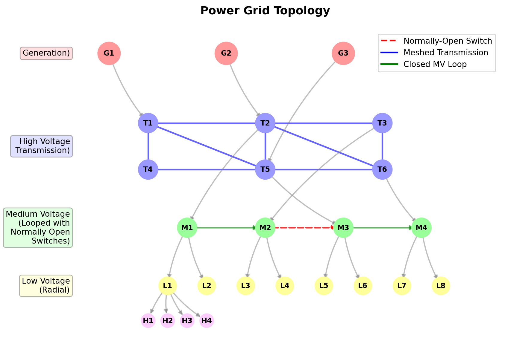
The transmission network is typically meshed, meaning there are multiple paths for power to flow between any two points. This provides redundancy and improves reliability, as power can be rerouted in the event of a line failure. In contrast, distribution networks are often radial, with a single path from the substation to each customer. This simplifies protection and control but can be less reliable if a line goes down. That is, a single fault can cut power to all downstream customers. Figure 1.13 illustrates these different topological characteristics at each voltage level.

Figure 1.13: Power grid topology showing multiple generators, meshed transmission network (multiple redundant paths), looped medium-voltage distribution with normally-open switches, and radial low-voltage distribution networks.

Note that the topology of the grid is not static; it can change due to maintenance, faults, or operational decisions. Grid operators use real-time monitoring and control systems to manage the topology and ensure reliable power delivery. At the transmission level, circuit breakers and switches can be used to isolate faults and reroute power as needed. In distribution systems, reclosers and sectionalizers help manage faults and restore service quickly. Moreover, protection systems are in place to detect faults and automatically disconnect affected sections of the grid to prevent damage and ensure safety. The simplest protection device is a fuse, which melts when current exceeds a certain level, breaking the circuit. More complex systems use relays and circuit breakers that can be remotely controlled and coordinated to isolate faults while minimizing disruption to the rest of the grid.

Imagine a high-voltage power transmission line that crosses over a motorway or freeway. If the line were to break, it would fall on the vehicles below, creating a dangerous situation. To prevent this, the line is equipped with protective devices that can detect faults (like a broken wire) and quickly disconnect the affected section of the line even before it falls to the ground (i.e., within a few tens of milliseconds). This prevents the fallen wire from energizing the vehicles below, reducing the risk of electric shock or accidents.

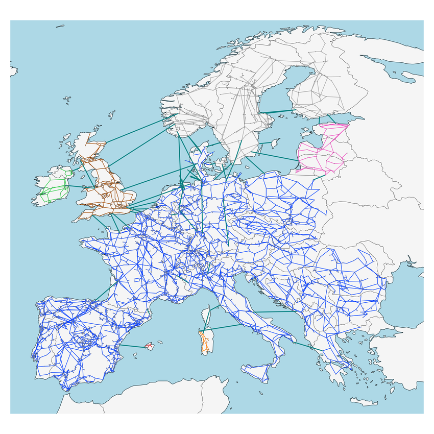
Each country usually has its own grid, with its own generators, transmission lines, and distribution systems. However, many countries are interconnected through high-voltage transmission lines, allowing them to share power and improve reliability. These interconnections can help balance supply and demand across larger regions, facilitate the integration of renewable energy sources, and provide backup power during emergencies. Trans-national grids, such as those in Europe, North America, and parts of Asia, are examples of such interconnections. They are increasingly important as the share of variable renewable energy sources grows, requiring greater flexibility and coordination across larger areas, as well as resilience against extreme weather events and other disruptions. Figure 1.14 shows the European electricity grid interconnections and synchronous areas.

Figure 1.14: Map of the European electricity grid showing interconnections and transmission lines. The European grid is highly interconnected, with multiple synchronous areas enabling cross-border power exchange and integration of renewable energy sources. Source: Hofmann et al. (2020), “Flow Allocation in Meshed AC-DC Electricity Grids,” DOI:10.20944/preprints202001.0352.v1

1.2.4 Loads

The purpose of a power grid is to deliver electricity to loads, which are devices or systems that consume electrical power. Loads can be broadly categorized into several types based on their characteristics and usage patterns:

Residential loads from homes are primarily for heating, cooling, and appliances such as refrigerators, washing machines and clothes dryers. Residential lighting used to be a significant load, but with the advent of energy-efficient LED lighting, its share has decreased. Residential loads tend to have daily and seasonal patterns, with well-defined peaks in the morning and evening when people are home. At night, loads drop significantly as people sleep (this is their base load). Seasonal variations are also significant, with higher loads in summer (due to air conditioning) and winter (due to heating), depending on geography. In many countries, which used to have winter peaks for heating, summer peaks have become more pronounced due to widespread adoption of air conditioning.
Commercial loads from businesses, offices, and retail establishments. These loads include heating, ventilation, and air conditioning (HVAC) systems, computers, and other office equipment. Commercial loads typically peak during business hours on weekdays and drop off in the evenings and weekends. They also have seasonal variations, particularly in regions with extreme temperatures that require significant heating or cooling.
Industrial loads from factories and manufacturing facilities. These loads can be very large and often operate continuously or in shifts. Industrial processes may include motors, furnaces, and other heavy machinery that consume significant amounts of power. Industrial loads can be more constant than residential or commercial loads, but they can also have specific patterns based on production schedules and processes.
Agricultural loads from irrigation systems, grain dryers, and other farming equipment. These loads can be seasonal and depend on agricultural cycles. Agricultural loads typically peak during planting and harvesting seasons, as well as during periods of high irrigation demand.
Municipal loads from street lighting, water treatment plants, and public transportation systems. These loads can have specific patterns based on municipal operations and services. Sewage treatment plants, for example, may have relatively constant loads, while street lighting peaks at night. Water pumping for municipal water supply and sewage can be a significant load.

Loads can also be classified in many other ways. For example, based on their electrical characteristics:

Resistive loads that consume power in proportion to the voltage and current (e.g., incandescent lighting, electric heaters).
Inductive loads that create a lag between voltage and current (e.g., motors, transformers).
Capacitive loads that create a lead between voltage and current (e.g., capacitor banks used for power factor correction).
Non-linear loads that draw current in a non-sinusoidal manner, causing harmonics in the power system (e.g., computers, LED lighting, variable frequency drives).

Based on their behavior and flexibility:

Dynamic loads that change their power consumption rapidly based on operating conditions (e.g., electric vehicles, HVAC systems with variable speed drives).
Static loads that have relatively constant power consumption over time (e.g., lighting, resistive heating).

From the perspective of grid management and reliability:

Critical loads that require uninterrupted power supply (e.g., hospitals, data centers).
Non-critical loads that can tolerate power interruptions or reductions (e.g., residential lighting, some industrial processes).

Based on their temporal patterns:

Base loads that run continuously and provide a constant demand on the grid (e.g., refrigeration, some industrial processes).
Peak loads that occur during specific times of the day or year when demand is highest (e.g., air conditioning during hot summer afternoons).
Intermittent loads that vary significantly over time due to external factors (e.g., electric vehicle charging based on user behavior).
Steady loads that have relatively constant consumption over time (e.g., lighting, resistive heating).
Cyclic loads that have regular patterns of consumption based on operational cycles (e.g., industrial processes with shift work).
Random loads that have unpredictable consumption patterns (e.g., residential loads influenced by human behavior).

Finally, in the context of demand response and grid flexibility (which we will study later), loads can be classified as:

Flexible or controllable loads that can be adjusted or shifted in time to help balance supply and demand on the grid (e.g., smart appliances, electric vehicle charging).
Inflexible loads that have fixed consumption patterns and cannot be easily adjusted (e.g., traditional lighting, some industrial processes).
Deferrable loads that can be postponed to a later time without significant impact (e.g., dishwashers, laundry machines).

Understanding the characteristics of different load types is essential for grid operators to manage supply and demand effectively, ensure reliability, and plan for future capacity needs.

An important characteristic of a load is its carbon intensity, which measures the amount of CO₂ emissions associated with the electricity consumed by that load. The carbon intensity of a load depends on the mix of generation sources supplying power to the grid at any given time. For example, if a load is served primarily by coal-fired power plants, its carbon intensity will be high, whereas if it is served by renewable energy sources like wind or solar, its carbon intensity will be low. Grid operators and policymakers use carbon intensity metrics to assess the environmental impact of electricity consumption and to design strategies for reducing emissions, such as promoting energy efficiency, demand response, and the integration of low-carbon generation sources. Energy informatics plays a key role in measuring, analyzing, and optimizing the carbon intensity of loads through advanced data analytics, real-time monitoring, and intelligent control systems, and we will explore these topics in more detail later in the book.

Key Concepts Review

In this section, we have studied the elements that make up a power grid, including generators, transmission and distribution networks, and loads. Now is a good time to check your understanding of these fundamental power grid concepts:

Power grid architecture and the four main components (generation, transmission, distribution, loads)
Electromagnetic induction and the principle of electric generators
Generator characteristics: synchronization, inertial response, real and reactive power
Ramp rates and their importance for grid flexibility
Carbon emissions from different generator types
Grid voltage levels: high voltage, medium voltage, and low voltage
Buses and branches as basic elements of grid topology
Grid topology: meshed transmission vs. radial distribution
Protection systems and their role in grid safety
Load types: residential, commercial, industrial, agricultural, and municipal
Load characteristics: resistive, inductive, capacitive, and non-linear
Load flexibility: flexible, inflexible, and deferrable loads
Carbon intensity of electricity consumption

1.3 Power Flow Analysis

Thus far, we’ve studied individual power system components—how generators produce power, how loads consume it, how transmission lines and transformers carry it, and how resistance and reactance affect current flow. But understanding individual components is only the first step. Real power grids contain hundreds or thousands of buses interconnected by transmission lines and transformers, forming complex networks. We now turn our attention to how these elements are combined to deliver power from generators to loads.

At a high level, this is akin to water from a reservoir being delivered to consumers. Unlike a water distribution system, however, where flow is primarily driven by pressure differences, the flow of electrical power in a grid is governed by more complex physical laws, specifically those described by Kirchhoff’s laws and Ohm’s law.

In a power grid, when you change something at one location—say, a generator increases output or a large factory suddenly starts its motors—the effects ripple throughout the entire network. You cannot simply apply Ohm’s law to individual components in isolation because the behavior at each point depends on the state of every other point in the network.

It is, therefore, necessary to use mathematical models and computational methods to analyze and predict power flows in the grid, i.e., how much electrical power is flowing through each transmission line and transformer in the network.

In this section, we will introduce the basic concepts and methods used in power flow analysis. Power flow analysis provides critical information for grid operators to ensure safe and efficient operation of the power system. It lets us answer practical questions like: What will happen to all bus voltages if a new solar farm comes online at bus 47? Which transmission line will reach its thermal limit first during peak demand? How much power flows through each of the 500 lines in the network right now? It also helps identify potential issues such as voltage violations (voltages exceeding nominal limit), line overloads, and instability, allowing operators to take corrective actions before problems arise. Additionally, power flow results are used in various optimization and planning studies to improve system performance and reliability.

1.3.1 Preliminaries: Per-Unit System

Before we can analyze power flows mathematically, we face a practical problem: power systems operate across wildly different scales. A residential outlet operates at 120 V, distribution lines at 12,000 V (12 kV), subtransmission at 69 kV, and high-voltage transmission at 345 kV or even 765 kV. Similarly, a household might draw 5 kW while an industrial facility consumes 50 MW—a factor of 10,000 difference. Working with such diverse magnitudes in the same calculation invites errors: Did I write 230,000 V or 2,300,000 V? Is this impedance 0.05 Ω at 345 kV or 50 Ω at 12 kV?

Even worse, when transformers connect systems at different voltage levels, the “same” physical power flow appears as vastly different voltage and current values on either side of the transformer. A 100 MW power flow might correspond to 290 A at 345 kV on the high-voltage side but 8,330 A at 12 kV on the low-voltage side. How do we write equations that work consistently across these transformations?

The solution is the per-unit system: a normalization technique that expresses all quantities (voltages, currents, powers, impedances) as dimensionless fractions of chosen reference values. It prevents numerical issues, makes magnitudes directly comparable, and simplifies calculations. In power systems, per-unit normalization is not optional; it’s the standard way professionals communicate and compute.

Per-unit normalization expresses electrical quantities (voltage, current, impedance, power) as a fraction or multiple of chosen base values. For any quantity $X$:

$X_{pu} = \frac{X_{actual}}{X_{base}}$

This method provides consistent, dimensionless values for all electrical quantities, greatly simplifying calculations—especially in complex networks with transformers, multiple voltage levels, and various equipment ratings.

1.3.1.1 Base Values and Derived Quantities

To use the per-unit system, we first select base values for voltage ($V_{base}$) and power ($S_{base}$), often chosen to match the rating of key equipment or a standard system voltage level. For example, at the distribution network (low voltage level), a typical value for the voltage base is 220V or 110V. We use apparent power ($S$) rather than real power ($P$) or reactive power ($Q$) as the base because this represents the total power capacity that equipment must be designed to handle, regardless of the power factor². From these base values, we derive other base quantities:

Base current (for three-phase systems): $I_{base} = \frac{S_{base}}{V_{base} \sqrt{3}}$
Base impedance: $Z_{base} = \frac{V_{base}^2}{S_{base}}$

Once base values are established, actual quantities are normalized:

Voltage: $V_{pu} = \frac{V_{actual}}{V_{base}}$
Current: $I_{pu} = \frac{I_{actual}}{I_{base}}$
Impedance: $Z_{pu} = \frac{Z_{actual}}{Z_{base}}$
Power: $S_{pu} = \frac{S_{actual}}{S_{base}}$

Example 1.7 Consider a system with $V_{base} = 220$ kV and $S_{base} = 100$ MVA. The base impedance is:

$Z_{base} = \frac{(220{,}000)^2}{100{,}000{,}000} = 484$ Ω

A transmission line with actual impedance $Z_{actual} = 4.84 + j24.2$ Ω becomes:

$Z_{pu} = \frac{4.84 + j24.2}{484} = 0.01 + j0.05$ p.u.

The per-unit value is much simpler to work with, especially when the system involves multiple voltage levels and transformers.

Throughout this chapter, we will use per-unit values for voltages, currents, impedances, and powers to simplify our power flow calculations.

1.3.2 A Metaphor for Power Flow

Power flow in an AC circuit can be challenging to understand because an alternating current flows both ways along a circuit, so a metaphor may help. Imagine a swing that is being pushed by a person standing at one end. The person injects power into the system to keep it moving at a certain frequency despite losses due to friction and air resistance. Now, suppose that another person standing at the other end places a pin that the swing hits just before it reaches its peak, so that the pin is knocked over. It should be evident that this additional dissipation of energy will require the person pushing the swing to exert more effort to maintain its motion. Moreover, this extra power is transferred by the swing to the other side. The further away the pin is placed from the top of the swing’s arc, the more the force with which it hits the pin, the more the mechanical work that is done, and the greater the power transfer.

In this metaphor, the person pushing the swing represents a generator injecting power into the grid, while the pin represents a load consuming power. The swing itself represents the transmission line that connects the generator and the load. Just as the generator injects power into the grid to maintain the amplitude of oscillation of the AC current, the swing is pushed to keep it moving at the same height. Similarly, just as the load consumes power from the grid, the pin is hit by the swing and causes it to perform mechanical work. The distance of the pin from the top of the swing’s arc represents the phase angle difference between the two ends of the transmission line, which affects the amount of power that can be transferred: the greater the angle difference, the more power can be transferred.

Just as the motion of the swing is influenced by factors beyond the control of the person pushing, such as air resistance and friction, the flow of power in the grid is influenced by the physical properties of the transmission lines, such as their resistance and reactance. The net power flow in the grid is determined by a combination of the generator’s output, the load’s consumption, and the characteristics of the transmission lines connecting them (such as resistance and reactance).

1.3.3 Power Flow on a Single Transmission Line

Let’s illustrate these concepts with a simple example with a single transmission line connecting two buses: Bus 1 with a generator that produces power and Bus 2 with a load that consumes power. The transmission line has a certain impedance (resistance and reactance) that affects how much power can flow between the two buses. We will also need to consider the voltage magnitudes and phase angles at each bus, as these will influence the power flow.

Note

Notation: In power systems analysis, the letter $j$ is used in two different ways: (1) as a subscript to denote a bus index (e.g., bus $i$, bus $j$), and (2) as the imaginary unit in complex numbers (e.g., $Z = R + jX$). While this dual usage follows standard conventions in the field, context makes the meaning clear: subscripts refer to buses, while $j$ standing alone represents $\sqrt{-1}$.

Also, in power systems analysis, when we write $V$ without any qualifier, it’s understood to be RMS voltage unless otherwise specified.

Let the two ends of a transmission line have RMS voltages $V_i$ and $V_j$ and the line have an impedance $Z_{ij} = R_{ij} + jX_{ij}$, where $R_{ij}$ is the resistance and $X_{ij}$ is the reactance due to inductive and capacitive elements on the line. Recall that the admittance ($Y_{ij}$) is the reciprocal of the impedance and is given by $Y_{ij} = G_{ij} + jB_{ij} =\frac{1}{Z_{ij}} = \frac{1}{R_{ij} + jX_{ij}} = \frac{R_{ij} - jX_{ij}}{R_{ij}^2 + X_{ij}^2}$, that conductance ($G_{ij}$) $=\frac{R_{ij}}{R_{ij}^2 + X_{ij}^2}$ is the real part of the admittance, and that susceptance ($B_{ij}$) $= -\frac{X_{ij}}{R_{ij}^2 + X_{ij}^2}$ is the imaginary part of the admittance.

1.3.3.1 Understanding What Drives Power Flow

Before presenting the mathematical formulas, let’s build intuition for what controls power flow between two buses:

Three Key Factors:

Voltage Magnitudes ($V_i$, $V_j$): Higher voltages at both ends create more potential for power transfer, similar to how higher water pressure in both connected tanks creates more flow potential. The product $V_i V_j$ appears in power flow equations—if either voltage is low, power transfer capability is reduced.
Angle Difference ($\theta_i - \theta_j$): This is the phase angle difference between the voltage phasors at the two buses. Remember from our swing metaphor: the further the swing moves from its peak before hitting the pin, the more power is transferred. Similarly, larger angle differences drive more real power flow. Think of angle difference as creating an “electrical slope” down which power flows.
Line Characteristics ($G_{ij}$, $B_{ij}$):
- Conductance ($G_{ij}$): Represents the line’s ability to conduct real power, analogous to pipe diameter in a water system. Higher conductance allows more power flow.
- Susceptance ($B_{ij}$): Related to reactive elements (inductance and capacitance) in the line. It affects reactive power flow and the relationship between voltage angles and power transfer.

Physical Insight: Real power flows primarily when there’s an angle difference between buses (like water flowing down a slope). Reactive power flows primarily when there’s a voltage magnitude difference (like water flowing from high pressure to low pressure). The line characteristics determine how easily power can flow for a given voltage and angle configuration.

Then, using Ohm’s law, the line current ($I_{ij}$) flowing from bus $i$ to bus $j$ is $I_{ij} = \frac{(V_i - V_j)}{R_{ij}} = Y_{ij} (V_i - V_j)$. The real and reactive power flows on the line are given by the fundamental power flow equations:

Power Flow Equations

$P_{ij} = V_i V_j (G_{ij} \cos(\theta_i - \theta_j) + B_{ij} \sin(\theta_i - \theta_j))$

$Q_{ij} = V_i V_j (G_{ij} \sin(\theta_i - \theta_j) - B_{ij} \cos(\theta_i - \theta_j))$

where:

$P_{ij}$ and $Q_{ij}$ are the active and reactive power flows from bus $i$ to bus $j$.
$V_i$ and $V_j$ are the voltage magnitudes at buses $i$ and $j$.
$\theta_i$ and $\theta_j$ are the voltage angles at buses $i$ and $j$.
$G_{ij}$ and $B_{ij}$ are the conductance and susceptance of the line connecting buses $i$ and $j$.

Where Do These Equations Come From?

These power flow equations derive from fundamental circuit analysis:

Ohm’s law for AC circuits: The current flowing between buses is $\vec{I}_{ij} = Y_{ij}(\vec{V}_i - \vec{V}_j)$, where $Y_{ij} = G_{ij} + jB_{ij}$ is the line admittance.
Power formula: Complex power is $\vec{S}_{ij} = \vec{V}_i \vec{I}_{ij}^*$ (where $*$ denotes complex conjugate).
Phasor representation: Expressing voltages as $\vec{V}_i = V_i e^{j\theta_i}$ and expanding using Euler’s formula yields the trigonometric terms.

The trigonometric functions arise from the phase relationships between voltage phasors. A complete step-by-step mathematical derivation is provided in the Appendix at the end of this section.

Note that the amount of power transferred depends on the difference in phase angles at the buses as well as the line characteristics (conductance and susceptance). If both ends of the line have the same power angle, then $B_{ij}$ term becomes zero, and the power flow is given simply by $V_i V_j (G_{ij})$. Note also that the power flow equations are nonlinear due to the trigonometric functions of the voltage angles.

1.3.3.2 Exploring Power Flow Dependencies

To build intuition for how different parameters affect power flow, let’s examine how real and reactive power change with varying angle differences and voltage magnitudes:

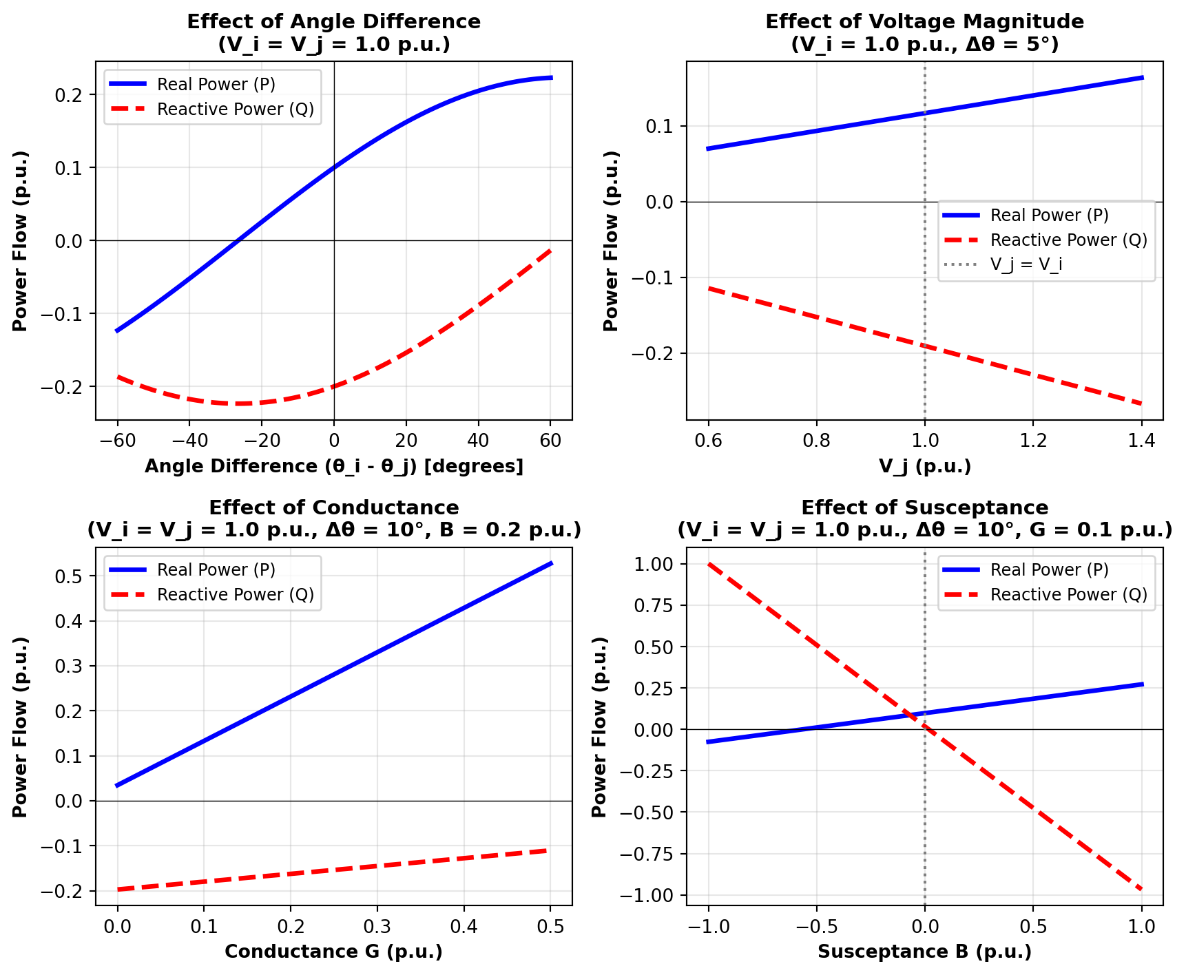
Figure 1.15: Sensitivity of real and reactive power flows to voltage angle difference (top) and voltage magnitude difference (bottom). These plots show how P and Q respond to changes in key parameters, with typical transmission line parameters (G = 0.1 p.u., B = 0.2 p.u.).

Note that power can flow in either direction depending on which bus has higher voltage/angle. The phase angle difference ($\theta_i - \theta_j$) drives the magnitude and direction of real power flow, while the voltage magnitude difference ($V_i - V_j$) primarily influences reactive power flow. Other key observations include:

Conductance (G) represents resistive losses; higher G means more real power can flow but there are also more losses due to the higher current and the quadratic dependence of loss on current.
A positive *susceptance (B)** typically represents inductive reactance. In typical transmission lines, B >> G, so that the reactive power transfer is quite small, making the angle-dependent term dominant for real power.

In the power flow equation $P_{ij} = V_i V_j [G_{ij}\cos(\theta_i - \theta_j) + B_{ij}\sin(\theta_i - \theta_j)]$, which parameter primarily drives the flow of real power: the voltage magnitude difference or the angle difference?
True or False: If two buses have voltages $V_1 = 1.0\angle 10°$ and $V_2 = 1.0\angle 10°$ (identical magnitude and angle), power will still flow between them if there is a load connected to bus 2.
Why are power flow equations called “nonlinear”?

Can’t answer confidently? Review the Power Flow Equations section and the visualization above.

The Slack Bus: Voltage Reference

Before analyzing multi-bus systems, we must understand a critical concept: the slack bus (also called swing bus or reference bus), which serves as the voltage reference point for the entire power system.

Power flow equations involve voltage angles ($\theta_i$, $\theta_j$, …). But angles are relative—only the difference between angles matters physically. This creates mathematical ambiguity: if $\theta_1 = 10°$, $\theta_2 = 30°$, $\theta_3 = 50°$ is a solution, then so is $\theta_1 = 0°$, $\theta_2 = 20°$, $\theta_3 = 40°$ (everything shifted by -10°). Both represent the same physical state because only the differences (20° between buses 1-2, and 30° between buses 1-3) affect power flow.

To remove this ambiguity, we fix one bus angle as the reference (typically 0°). This is analogous to: - Defining “ground” as 0V in a DC circuit - Choosing Greenwich, England as 0° longitude on Earth - Setting Unix epoch as time reference (Jan 1, 1970 = time zero)

Slack Bus Responsibilities:

Voltage Angle Reference: $\theta_{slack} = 0°$ (by definition—this is our angular reference point)
Voltage Magnitude: $V_{slack}$ is typically fixed at 1.0 p.u. (nominal voltage), though it can be specified at other values
Balances Power Mismatches: The slack bus generator adjusts its output to exactly match total demand plus losses. Since losses aren’t known until after we solve the power flow equations, we can’t specify the slack bus power output in advance—it’s determined by the solution.

Typically, we choose a slack bus to be a bus with: - A large, flexible generator (can absorb power mismatches without violating limits) - Central location in the network (electrically close to most loads) - Stable voltage control capability

Often, this is the largest power plant or a major transmission hub.

Bus Types

In power flow analysis, buses are classified into three types:

Slack Bus (Reference Bus): Voltage magnitude $V$ and angle $\theta$ are fixed (known). Real power $P$ and reactive power $Q$ are unknowns (determined by solving to balance the system).
PV Buses (Generator Buses): Real power $P$ and voltage magnitude $V$ are specified (known). Reactive power $Q$ and angle $\theta$ are unknowns (to be solved).
PQ Buses (Load Buses): Real power $P$ and reactive power $Q$ are specified (known). Voltage magnitude $V$ and angle $\theta$ are unknowns (to be solved).

This is because generators can control their voltage magnitude (through excitation control) and real power output (through prime mover control), so these are specified. The slack bus is special—we let it absorb all power mismatches, so its power output floats. Loads consume fixed amounts of power but can’t control voltage, so voltage is what we solve for.

1.3.4 Power Flow in a Three-bus Network

We now consider a more complex example involving a three-bus power system with one generator and two loads as shown in Figure 1.16.

Figure 1.16: Simple three-bus power system with one generator (Bus 1) and two loads (Bus 2 and Bus 3). The generator supplies power to the loads through transmission lines with specified impedances. Buses are represented using standard electrical notation as thick horizontal lines.

Bus Classification and Known/Unknown Quantities:

Bus 1 (Slack Bus / Generator): Large generator serving as voltage reference
- $V_1 = 1.0$ p.u. (fixed - nominal voltage)
- $\theta_1 = 0°$ (fixed - reference angle)
- $P_G$ = $P_1$ is unknown (generator output to be determined)
- $Q_G$ = $Q_1$ is unknown (reactive power to be determined)
Bus 2 (PQ Bus / Load): Consumer load
- $P_{L2}$ is specified (known load consumption, treated as negative injection)
- $Q_{L2}$ is specified (known reactive power consumption)
- $V_2$ is unknown (voltage magnitude to be solved)
- $\theta_2$ is unknown (voltage angle to be solved)
Bus 3 (PQ Bus / Load): Consumer load
- $P_{L3}$ is specified (known load consumption)
- $Q_{L3}$ is specified (known reactive power consumption)
- $V_3$ is unknown (voltage magnitude to be solved)
- $\theta_3$ is unknown (voltage angle to be solved)
Transmission Lines: All line impedances $Z_{12}$, $Z_{13}$, and $Z_{23}$ are known

Analyzing the power flow in this system means determining all the unknown values: the slack bus power output ($P_1$, $Q_1$), voltage magnitudes at load buses ($V_2$, $V_3$), voltage angles ($\theta_2$, $\theta_3$), as well as the active and reactive power flows on each transmission line. This is done by solving a set of simultaneous nonlinear equations based on Ohm’s and Kirchhoff’s laws, while taking into account the impact of line parameters on power flow.

To begin with, here are the power flow equations for each bus, which basically express the balance of power at each bus (i.e., power injected minus power consumed equals zero):

Bus 1 (Generator Bus):
- Active Power Balance: $P_G - P_{12} - P_{13} = 0$
- Reactive Power Balance: $Q_G - Q_{12} - Q_{13} = 0$
Bus 2 (Load Bus):
- Active Power Balance: $-P_{L2} + P_{21} + P_{23} = 0$
- Reactive Power Balance: $-Q_{L2} + Q_{21} + Q_{23} = 0$
Bus 3 (Load Bus):
- Active Power Balance: $-P_{L3} + P_{31} + P_{32} = 0$
- Reactive Power Balance: $-Q_{L3} + Q_{31} + Q_{32} = 0$

These equations are written in terms of the power flow on each line, which are calculated using the equations similar to the ones used in the two-bus case. For example, the active and reactive power flows from Bus 1 to Bus 2 are given by:

$P_{12} = V_1 V_2 (G_{12} \cos(\theta_1 - \theta_2) + B_{12} \sin(\theta_1 - \theta_2))$
$Q_{12} = V_1 V_2 (G_{12} \sin(\theta_1 - \theta_2) - B_{12} \cos(\theta_1 - \theta_2))$

We can write the power flow equations for the other lines ($P_{13}$, $Q_{13}$, $P_{23}$, $Q_{23}$) using the same formulas. Substituting these values into the power balance equations, we define a system of six nonlinear equations,

Recall that the knowns in these equations are the power injections and line parameters ($B_{12}$,$G_{12}$, $B_{13}$,$G_{13}$ , $B_{23}$,$G_{23}$) and the six unknowns are the voltage magnitudes ($V_1$, $V_2$, $V_3$) and angles ($\theta_1$, $\theta_2$, $\theta_3$) at each bus. Thus, we have six equations which allow us to find six unknowns. The solution to this system of equations gives us the voltage profile of the network as well the active and reactive power flows on each transmission line.

1.3.5 Solution Approach: Newton-Raphson Method

The typical way to solve this set of nonlinear equations is to use iterative numerical methods, such as the Newton-Raphson method. These methods start with an initial guess for the bus voltages and angles and iteratively refine the estimates, focusing on the mismatch between the known and guessed active and reactive power values until convergence is achieved (i.e., the changes in bus voltages and angles are below a specified tolerance). From a CS perspective, this is similar to gradient descent in machine learning—both iteratively improve an initial guess by computing gradients (or Jacobians in this case) and taking steps toward the solution, though Newton-Raphson typically converges much faster (3-5 iterations vs. thousands) due to its use of second-order information. The steps are as follows:

Initialization: Start with an initial guess for bus voltages and angles (e.g., all voltages at 1.0 p.u. and phase angles of 0 degrees).
Formulate Mismatch Equations: Next, we calculate the power mismatches (differences between specified and calculated power injections) at each bus. In our example, we compute the mismatches for active and reactive power at each bus based on the current voltage estimates. Specifically, we have six mismatch equations (two for each bus). These are:
- Bus 1:
  - $\Delta P_1 = P_G - (P_{12} + P_{13})$
    - This indicates the difference between the generated power and the sum of power flows to buses 2 and 3.
  - $\Delta Q_1 = Q_G - (Q_{12} + Q_{13})$
    - Similarly, this indicates the difference between the generated reactive power and the sum of reactive power flows to buses 2 and 3.
- Bus 2:
  - $\Delta P_2 = -P_{L2} + (P_{21} + P_{23})$
    - For the load bus, this indicates the difference between the consumed power and the sum of power flows from buses 1 and 3.
  - $\Delta Q_2 = -Q_{L2} + (Q_{21} + Q_{23})$
    - And similarly for reactive power.
- Bus 3:
  - $\Delta P_3 = -P_{L3} + (P_{31} + P_{32})$
  - $\Delta Q_3 = -Q_{L3} + (Q_{31} + Q_{32})$
Construct Jacobian Matrix: Build the Jacobian matrix that holds the partial derivatives of the power mismatches with respect to voltage magnitudes and angles at each bus. Specifically, the Jacobian matrix $J$ can be structured as follows (see below for an example):
1. $\frac{\partial \Delta P_i}{\partial \theta_j}$: Partial derivatives of active power mismatches with respect to voltage angles.
2. $\frac{\partial \Delta P_i}{\partial V_j}$: Partial derivatives of active power mismatches with respect to voltage magnitudes.
3. $\frac{\partial \Delta Q_i}{\partial \theta_j}$: Partial derivatives of reactive power mismatches with respect to voltage angles.
4. $\frac{\partial \Delta Q_i}{\partial V_j}$: Partial derivatives of reactive power mismatches with respect to voltage magnitudes.
Formulate Linear System: To set up a linear system to solve one step of the Newton-Raphson iteration, we first linearize the nonlinear power flow equations using a first-order Taylor series expansion. For readers who have not seen this technique before, the intuition is that if we have a nonlinear function $f(x)$ and we want to find $x$ such that $f(x) = 0$, we can approximate $f(x + \Delta x) \approx f(x) + J \Delta x$, where $J$ is the Jacobian matrix of partial derivatives. Setting $f(x + \Delta x) = 0$ and solving for $\Delta x$ gives $\Delta x = -J^{-1} f(x)$, or equivalently, $J \Delta x = -f(x)$. In our case, $f(x)$ represents the power mismatch vector $\begin{bmatrix} \Delta P \\ \Delta Q \end{bmatrix}$, and $x$ represents the bus voltages and angles. The mismatch vector contains all the $\Delta P_i$ values stacked on top of all the $\Delta Q_i$ values. By solving this linear system and updating our estimates as $x_{new} = x_{old} + \Delta x$, we converge toward the solution where all power mismatches are zero. For our example, here is the linear system equations to solve at each iteration: \[ \begin{bmatrix} \frac{\partial \Delta P_1}{\partial \theta_1} & \frac{\partial \Delta P_1}{\partial \theta_2} & \frac{\partial \Delta P_1}{\partial \theta_3} & \frac{\partial \Delta P_1}{\partial V_1} & \frac{\partial \Delta P_1}{\partial V_2} & \frac{\partial \Delta P_1}{\partial V_3} \\ \frac{\partial \Delta P_2}{\partial \theta_1} & \frac{\partial \Delta P_2}{\partial \theta_2} & \frac{\partial \Delta P_2}{\partial \theta_3} & \frac{\partial \Delta P_2}{\partial V_1} & \frac{\partial \Delta P_2}{\partial V_2} & \frac{\partial \Delta P_2}{\partial V_3} \\ \frac{\partial \Delta P_3}{\partial \theta_1} & \frac{\partial \Delta P_3}{\partial \theta_2} & \frac{\partial \Delta P_3}{\partial \theta_3} & \frac{\partial \Delta P_3}{\partial V_1} & \frac{\partial \Delta P_3}{\partial V_2} & \frac{\partial \Delta P_3}{\partial V_3} \\ \frac{\partial \Delta Q_1}{\partial \theta_1} & \frac{\partial \Delta Q_1}{\partial \theta_2} & \frac{\partial \Delta Q_1}{\partial \theta_3} & \frac{\partial \Delta Q_1}{\partial V_1} & \frac{\partial \Delta Q_1}{\partial V_2} & \frac{\partial \Delta Q_1}{\partial V_3} \\ \frac{\partial \Delta Q_2}{\partial \theta_1} & \frac{\partial \Delta Q_2}{\partial \theta_2} & \frac{\partial \Delta Q_2}{\partial \theta_3} & \frac{\partial \Delta Q_2}{\partial V_1} & \frac{\partial \Delta Q_2}{\partial V_2} & \frac{\partial \Delta Q_2}{\partial V_3} \\ \frac{\partial \Delta Q_3}{\partial \theta_1} & \frac{\partial \Delta Q_3}{\partial \theta_2} & \frac{\partial \Delta Q_3}{\partial \theta_3} & \frac{\partial \Delta Q_3}{\partial V_1} & \frac{\partial \Delta Q_3}{\partial V_2} & \frac{\partial \Delta Q_3}{\partial V_3} \end{bmatrix} \begin{bmatrix} \Delta \theta_1 \\ \Delta \theta_2 \\ \Delta \theta_3 \\ \Delta V_1 \\ \Delta V_2 \\ \Delta V_3 \end{bmatrix} = - \begin{bmatrix} \Delta P_1 \\ \Delta P_2 \\ \Delta P_3 \\ \Delta Q_1 \\ \Delta Q_2 \\ \Delta Q_3 \end{bmatrix} \]
Solve Linear System: Solve this system to give us the updates $\Delta \theta_i$ and $\Delta V_i$ to apply to our voltage estimates.
Update Variables: Update bus voltages and angles using the calculated changes.
Check Convergence: Repeat steps 2-6 until the power mismatches are within the specified tolerance or the maximum number of iterations is reached. At each iteration, we update the voltage estimates by:

$\theta_i^{new} = \theta_i^{old} + \Delta \theta_i$
$V_i^{new} = V_i^{old} + \Delta V_i$

Once convergence is achieved, the final results provide the voltage magnitudes and angles at each bus (the converged values after all iterations as well as the power flows on each transmission line, calculated using the final voltage and angle values and the power flow equations Detailed calculations and iterations are typically performed using specialized software or programming languages (e.g., Python, MATLAB) due to the complexity of the equations involved.

The steps outlined above provide a basic framework for performing power flow analysis in a simple three-bus system. In practice, power systems can be much more complex, with many buses, generators, loads, and transmission lines. However, the fundamental principles and methods remain the same, allowing engineers to analyze and optimize the operation of large-scale power grids effectively.

1.3.6 Line Constraints and Losses

In the discussion so far, we have assumed that transmission lines can carry any amount of power without limitations. In reality, however, transmission lines have physical constraints that limit the amount of power they can safely carry. These constraints are typically defined by thermal limits (maximum current capacity), voltage limits (minimum and maximum voltage levels), and stability limits (maximum angle difference between buses). Additionally, transmission lines experience losses due to their resistance, which results in a portion of the transmitted power being dissipated as heat. These losses can be calculated using the formula:

$P_{loss} = I^2 R$

where $I$ is the current flowing through the line and $R$ is the resistance of the line. In power flow analysis, these losses must be accounted for to ensure accurate calculations of power flows and system performance (i.e., the power generated must equal the power consumed plus losses).

When performing power flow analysis, it is essential to consider these constraints to ensure that the calculated power flows do not exceed the line limits. What happens if a line is overloaded or if losses are too high? In such cases, the power flow analysis may indicate that the system is operating outside of its safe limits. Operators may need to take corrective actions, such as redistributing power flows, adjusting generation levels, or implementing demand response (load reduction) measures to reduce load.

1.3.7 Optimal Power Flow (OPF)

In the system described above, there is a single generator supplying power to the loads. In real-world power systems, there are often multiple generators with different cost structures and operational constraints. The goal of optimal power flow (OPF) is to determine the optimal operating conditions for all generators in the system while minimizing the total generation cost and satisfying all system constraints (e.g., power balance, line limits, voltage limits). The OPF problem can be formulated as a constrained optimization problem, where the objective function is the total generation cost, and the constraints include the power flow equations, generator limits, and line limits. The solution to the OPF problem provides the optimal generation levels for each generator, as well as the voltage profile and power flows in the system. In practice, the OPF problem also includes line constraints and losses, making it a more complex optimization problem that requires advanced numerical methods to solve.

The generic formulation of the OPF problem is as follows:

Minimize: $C = \sum_{i=1}^{N_G} C_i(P_{Gi})$
Subject to:

Power flow equations at each bus
Generator limits: $P_{Gi}^{min} \leq P_{Gi} \leq P_{Gi}^{max}$, $Q_{Gi}^{min} \leq Q_{Gi} \leq Q_{Gi}^{max}$
Line limits: $|S_{ij}| \leq S_{ij}^{max}$
Voltage limits: $V_i^{min} \leq V_i \leq V_i^{max}$
Other system constraints as needed

Where:

$C$ is the total generation cost.
$C_i(P_{Gi})$ is the cost function for generator $i$ as a function of its active power output $P_{Gi}$.
$N_G$ is the number of generators in the system.
$P_{Gi}^{min}$, $P_{Gi}^{max}$, $Q_{Gi}^{min}$, and $Q_{Gi}^{max}$ are the minimum and maximum active and reactive power limits for generator $i$.
$S_{ij}$ is the apparent power flow on line $ij$.
$S_{ij}^{max}$ is the maximum allowable apparent power flow on line $ij$.
$V_i^{min}$ and $V_i^{max}$ are the minimum and maximum voltage limits at bus $i$.

Note

Other constraints may be added depending on the specific requirements of the power system being analyzed. These include generator ramp rates, minimum generator up/down times, and reserve requirements (i.e., availability of excess generation capacity in case of an unexpected event such as a line loss or a generator loss), as well as environmental constraints such as emissions limits. Solving the OPF problem typically requires advanced optimization techniques, such as interior-point methods, genetic algorithms, or particle swarm optimization, due to the nonlinear and non-convex nature of the problem. We will explore some of these techniques in later chapters.

Key Concepts Review

In this section, we introduced the per-unit system as a method to simplify power system analysis by normalizing electrical quantities. We discussed how to select base values for voltage and power, and how to derive base current and impedance. We then explored the fundamental power flow equations for a single transmission line, highlighting the dependencies of real and reactive power flows on voltage magnitudes and phase angles. Now is a good time to check your understanding of these fundamental power system analysis concepts:

Per-unit system and normalization of electrical quantities
Base values for voltage, power, current, and impedance
Power flow equations for transmission lines
Conductance and susceptance and their role in power flow
Voltage magnitude and phase angle dependencies
Three-bus power system analysis
Newton-Raphson method for solving power flow equations
Jacobian matrix and iterative solution techniques
Line constraints and losses in power systems
Optimal Power Flow (OPF) problem formulation

1.4 Grid Operations

In this section, we outline how a power grid is operated, typically by a grid operator (also called the Transmission System Operator or TSO, or Independent System Operator or ISO) who is responsible for maintaining the integrity of the grid. We will examine the key aspects of grid operations: balancing supply and demand through hierarchical control, market-based approaches to grid balance by coordinating economic dispatch and unit commitment, maintaining operating reserves to ensure power system security, and regulating grid operations.

1.4.1 Grid Balancing

At the most basic level, the role of a grid operator is to match generation and load. If they do not more or less match, then the frequency of the alternating current (also called the grid frequency) changes: it goes above the nominal 50/60 Hz value if supply exceeds demand and below it otherwise. There is a similar impact on voltages, with over-voltage or under-voltage at some buses. A large deviation from the nominal values can cause extensive damage to equipment and must be avoided as far as possible.

Balancing the grid is a fiendishly complex task! If someone turns on a light switch somewhere, then some generator, perhaps hundreds of kilometers away, needs to inject more power into the network, and it needs to make its way to the load. Moreover, the grid needs to provide power despite major swings in usage between day and night, working and non-working days, and despite failures in generators, lines, transformers and other grid elements. Reliable grid power that conforms to its nominal frequency and voltage limits is a daily miracle that most people take for granted, but is only achieved through some marvels of engineering. Although the details are far too complex to be covered in an introductory text, this section will attempt to capture some high level approaches needed for maintaining grid balance.

Making sure that there is enough supply to match anticipated demand requires actions and planning at several time scales:

At the level of years or decades, the grid operator will need to forecast demand changes due to effects such as appliance penetration (such as the increasing use of air conditioning and electric vehicles around the world), population growth, and industrialization and deindustrialization so that generation capacity, which takes years to build, can be planned out.
At the scale of months, they must forecast the expected load for the coming year, so that purchases of electricity from neighboring grids can be made, if needed.
At the scale of a day, they need to forecast the demand the next day, so that potential suppliers can get their plants ready in time.
At the scale of hours, they need to choose which generators to run, and at what power level, to minimize cost and achieve other goals such as carbon footprint minimization.
At the scale of minutes, they need to activate generator reserves to meet nominal limits on voltage and frequency.
Finally, at the fastest timescale of seconds and faster, they need to instantaneously control slack buses (typically synchronous generators) so that the total active and reactive power in the network matches the total load and line losses.

Here, we will study hierarchically structured control actions at the seconds, minutes, and hours levels, which are often called primary, secondary, and tertiary controls, respectively.

1.4.1.1 Primary Control (Frequency Matching)

At the fastest timescale (0-30 seconds), primary control is responsible for rapidly responding to load changes. Importantly, this is done independently at each generator, rather than being centrally coordinated.

For rotating generators, a certain degree of primary control is available automatically from what is known as the droop response, where the prime mover (water, steam, or a mechanical source) does a bit more work when the grid frequency drops due to an increase in load. In such systems, a governor senses a slight drop in frequency and automatically increases the generator’s power (for example, by opening a steam valve more widely) to maintain grid frequency. This action is carried out at all generators in parallel, and requires some extra generation capacity to be set aside as a primary reserve. However, inverter-based renewables do not have the inherent mechanical inertia of synchronous generators, so renewables-heavy grids need additional frequency support mechanisms such as synthetic inertia and fast frequency response from battery storage or wind/solar curtailment reserves, a topic we will return to later.

1.4.1.2 Secondary Control (Frequency Restoration)

Unlike primary control, which is decentralized and implemented independently at each generator, secondary control is a centralized automatic regulation carried out by the grid operator through Automatic Generation Control (AGC). Operating on a timescale of tens of seconds to minutes (typically 30 seconds to 15 minutes), secondary control has two main objectives: first, to restore system frequency to its nominal value (50 or 60 Hz) after primary reserves have responded to the frequency deviation; and second, to correct errors in previously scheduled tie-line power exchanges between interconnected control areas. These are exchanges between peer power grids controlled by different operators to make up for shortfalls. Corrective actions taken by primary controllers could cause persistent shortfalls in tie-lines, which secondary control accounts for.

AGC continuously monitors the Area Control Error (ACE), which combines frequency deviation and tie-line flow errors, and sends setpoint adjustments to selected generators to drive ACE back to zero. By restoring frequency to nominal and rebalancing inter-area power flows, secondary control lets the primary reserves that responded to the initial disturbance recover, preparing them to respond to the next contingency. The generators participating in secondary control are typically chosen based on their ability to respond quickly and to optimize objectives such as minimizing cost or carbon emissions.

1.4.1.3 Tertiary Control (Replacement Reserve)

While primary and secondary controls focus on immediate frequency stabilization, tertiary control is initiated manually or semi-automatically by grid operators. Tertiary control focuses on economic optimization and reserve management rather than fast frequency recovery and operates on an even longer timescale of 15 minutes to several hours. It tries to restore the reserves that were depleted during secondary control actions. Its primary purpose is to reallocate generation among power plants, start up or shut down generating units as needed (rather than simply changing setpoints), and restore reserve margins to prepare the system for future disturbances. Service providers participating in tertiary control must be able to deliver the requested reserve capacity within specified time limits (often 30 minutes) and at minimum ramp rates (typically 2 MW/min or higher).

Comparison: Grid Control Hierarchy

Control Level	Timescale	Control Type	Sensor Input	Actuator Output	Objective	Example Action
Primary (Automatic)	0-30 seconds	Decentralized (local at each generator)	Generator shaft speed/ grid frequency	Governor position (fuel/steam flow rate)	Arrest frequency deviation (stop the fall/rise)	Frequency drops from 60.00 Hz to 59.85 Hz → governors at all generators automatically open steam valves proportionally via droop response
Secondary (AGC)	30 sec - 15 min	Centralized (system-wide coordination)	Area Control Error (ACE) (frequency + tie-line flows)	Generator power setpoints (MW adjustments)	Restore nominal frequency (60.00 Hz) and correct tie-line flow errors	AGC sends commands: Plant A increase by +50 MW, Plant B decrease by -30 MW to drive ACE to zero
Tertiary (Economic)	15 min - hours	Manual or semi-automatic (operator decisions)	Load forecasts, reserve levels, market prices	Unit commitment decisions (start/stop generators)	Optimize economics, restore depleted reserves	Operator commits a quick-start gas turbine to replace spinning reserve used by secondary control

1.4.2 The Electricity Market

We now understand how the grid maintains balance between supply and demand through hierarchical control—primary control stabilizes frequency within seconds, secondary control restores nominal frequency within minutes, and tertiary control handles longer-term adjustments. But this raises an important question: When tertiary control needs to adjust generator outputs to match forecasted demand, which generators should be increased or decreased, and by how much?

The naive approach would be to split demand equally among all available generators. But power generators have vastly different operating costs: a nuclear plant might produce electricity for $25/MWh, a coal plant for $40/MWh, a natural gas plant for $60/MWh, and an oil-fired peaker plant for $150/MWh. Running all generators equally would waste money—we’d be using expensive generation when cheaper capacity is available. Even worse, generator costs aren’t fixed—each generator has a marginal cost curve where producing additional power becomes increasingly expensive as it approaches maximum capacity.

For a 20 GW power system, which is typical for a medium-sized country, a 1% improvement in generator dispatch efficiency translates to millions of dollars in savings per week. Over a year, suboptimal dispatch could waste billions of dollars and unnecessarily increase emissions. This is where unit commitment and economic dispatch come in: mathematical optimization problems that determine which generators to commit (turn on) and how to allocate demand among them to minimize total cost while respecting physical constraints. These aren’t just academic exercises—they’re the core computational problems that grid operators solve thousands of times per day to keep electricity affordable and reliable.

The coordination between these two problems occurs through the two-settlement system: generators commit to supply schedules in the day-ahead market and receive payments at day-ahead prices, then any deviations from these schedules are settled in the real-time market at real-time prices, where economic dispatch continuously adjusts output levels among committed generators to match actual demand. This structure provides both financial certainty for generators (who know a day ahead whether they’ll run) and operational flexibility for grid operators to balance supply and demand in real time.

Let us now look into each mechainsm in more detail.

1.4.2.1 Unit Commitment

Unit commitment refers to the advance commitment of a generation unit to supplying power. Generator owners respond to market requests (described in more detail below) and commit their unit to produce power to meet an anticipated demand. The result of unit commitment is the decision to have a generator turned on or off for some future time period, usually a few hours or a day ahead. This allows time for the generator operator to turn on the generator and ramp up its power generation. Unit commitment may require the operator (on behalf of the consumers) to pay for start-up and shut-down costs as well as a payment even if the generator is not actually used. The latter case arises when the operator schedules operating reserves, that is, generation capacity that is available in case the load exceeds its forecast.

The unit commitment problem must account for these temporal constraints while minimizing total system cost over the planning horizon, including both startup/shutdown costs and ongoing generation costs. A generator with low marginal cost might still not be worth committing if demand will only exceed its minimum stable generation level for a short period, making the startup cost economically unjustifiable.

In fully- or partially-deregulated electricity markets, unit commitment is coordinated with market clearing mechanisms through the day-ahead market. Generators submit multi-part bids that include not only their willingness to supply power at different price levels (their supply curves) but also their startup costs, minimum/maximum generation levels, and ramping capabilities. The market operator uses these bids to solve the unit commitment problem, determining which generators to commit for each hour of the next day.

1.4.2.2 Economic Dispatch

Once the unit commitment decisions have been made, that is, once we know which generators will be running, the next challenge is to determine how much power each committed generator should produce to meet the total system demand at minimum cost. This problem is known as economic dispatch. Economic dispatch operates on a shorter timescale than unit commitment, typically solving an optimization problem (which includes solving an optimal power flow problem) every 5 to 15 minutes, and assumes that the set of available generators is fixed, and their generation capacity is known. From a CS perspective, this is a constrained optimization problem—mathematically equivalent to quadratic programming or linear programming (depending on cost function form)—that you might solve using libraries like SciPy’s optimize module, CVXPY, or Google OR-Tools.

The fundamental principle underlying economic dispatch is simple: to minimize total generation cost, we should increase production from generators with lower marginal costs (lower costs of producing one additional unit of power) and decrease production from generators with higher marginal costs, subject to each generator’s capacity limits and other operational constraints.

Merit Order and Marginal Cost Curves

Each generator has a cost curve that relates its power output to the total cost of production. For thermal generators (coal, gas, nuclear), this curve is typically convex³ and increasing, reflecting the fact that it becomes progressively more expensive to extract additional power as the generator approaches its maximum capacity. The marginal cost at any operating point is the derivative of this cost curve—it represents the incremental cost of producing one more megawatt of power.

The merit order is a ranking of all available generators by their marginal costs at current operating points. In its simplest form, economic dispatch follows merit order: cheaper generators run at full capacity first, and progressively more expensive generators are brought online until total generation meets demand. This creates a merit order curve or supply curve that shows the cumulative capacity available at each price level. The point where this supply curve intersects the demand level determines the marginal price of electricity—the cost of the most expensive generator needed to meet demand. Importantly, all suppliers are paid this marginal price, which may appear to be fair, but can result in substantial profits for renewables-based generators, who have no fuel cost.

Figure 1.17: Merit order curve showing generators ranked by marginal cost. Cheaper generators (renewables, nuclear) are dispatched first, followed by progressively more expensive generators (coal, gas) until total capacity meets demand. The clearing price is set by the marginal generator.

Equal Incremental Cost Criterion

While merit order provides intuition, the mathematically optimal solution to economic dispatch is given by the equal incremental cost criterion (also called the equal lambda condition). This principle states that at the optimal dispatch, all generators that are not at their capacity limits must have equal marginal costs.

To see why, suppose two generators have different marginal costs—say generator A has a marginal cost of $30/MWh and generator B has a marginal cost of $40/MWh. We could reduce total cost by decreasing B’s output by 1 MWh (saving $40) and increasing A’s output by 1 MWh (costing $30), yielding a net savings of $10. This arbitrage opportunity persists until the marginal costs equalize. The common marginal cost at optimality, often denoted $\lambda$ (lambda), represents the system marginal cost—the cost of serving one additional megawatt of demand.

Mathematically, if generator i has a cost function $C_i(P_i)$ where $P_i$ is its power output, the economic dispatch problem is:

minimize $\sum C_i(P_i)$

subject to: $\sum P_i = P_{demand}$

$P_i^{min} ≤ P_i ≤ P_i^{max} for all i$

The Lagrangian optimality conditions yield $dC_i/dP_i = \lambda$ for all generators not at their limits, which is precisely the equal incremental cost criterion.

Example 1.8 Problem: A power system has three generators supplying a total demand of 150 MW. Each generator has a quadratic cost function:

Generator 1: $C_1(P_1) = 500 + 10P_1 + 0.05P_1^2$ ($/hr)
Generator 2: $C_2(P_2) = 400 + 12P_2 + 0.04P_2^2$ ($/hr)
Generator 3: $C_3(P_3) = 300 + 15P_3 + 0.03P_3^2$ ($/hr)

Operating limits: $10 \leq P_i \leq 80$ MW for all generators.

Find the optimal economic dispatch that minimizes total generation cost while meeting demand.

Solution:

Step 1: Calculate Marginal Costs

The marginal cost (incremental cost) for each generator is the derivative of its cost function:

$\frac{dC_1}{dP_1} = 10 + 0.10P_1$ ($/MWh)
$\frac{dC_2}{dP_2} = 12 + 0.08P_2$ ($/MWh)
$\frac{dC_3}{dP_3} = 15 + 0.06P_3$ ($/MWh)

Step 2: Apply Equal Incremental Cost Criterion

At the optimal dispatch (assuming no generators are at limits), all marginal costs must be equal to the system marginal cost $\lambda$:

\[10 + 0.10P_1 = 12 + 0.08P_2 = 15 + 0.06P_3 = \lambda\]

Step 3: Set Up the System of Equations

From the equal marginal cost conditions:

$10 + 0.10P_1 = 12 + 0.08P_2$ → $0.10P_1 - 0.08P_2 = 2$
$12 + 0.08P_2 = 15 + 0.06P_3$ → $0.08P_2 - 0.06P_3 = 3$

Plus the demand constraint: - $P_1 + P_2 + P_3 = 150$

Step 4: Solve for Generator Outputs

From the first equation: $P_1 = 20 + 0.8P_2$

From the second equation: $P_2 = 37.5 + 0.75P_3$

Substituting into the demand constraint:

\[(20 + 0.8P_2) + P_2 + P_3 = 150\] \[20 + 0.8(37.5 + 0.75P_3) + (37.5 + 0.75P_3) + P_3 = 150\] \[20 + 30 + 0.6P_3 + 37.5 + 0.75P_3 + P_3 = 150\] \[87.5 + 2.35P_3 = 150\] \[P_3 = 26.6 \text{ MW}\]

Back-substituting:

\[P_2 = 37.5 + 0.75(26.6) = 57.5 \text{ MW}\] \[P_1 = 20 + 0.8(57.5) = 66.0 \text{ MW}\]

Step 5: Verify Constraints

Check operating limits:

$P_1 = 66.0$ MW ✓ (within 10-80 MW)
$P_2 = 57.5$ MW ✓ (within 10-80 MW)
$P_3 = 26.6$ MW ✓ (within 10-80 MW)

Check demand: $66.0 + 57.5 + 26.6 = 150$ MW ✓

Step 6: Calculate System Marginal Cost

\[\lambda = 10 + 0.10(66.0) = 16.6 \text{ \$/MWh}\]

Verify for all generators:

Generator 1: $10 + 0.10(66.0) = 16.6$ $/MWh ✓
Generator 2: $12 + 0.08(57.5) = 16.6$ $/MWh ✓
Generator 3: $15 + 0.06(26.6) = 16.6$ $/MWh ✓

Step 7: Calculate Total Cost

\[C_{total} = C_1(66.0) + C_2(57.5) + C_3(26.6)\] \[= [500 + 10(66.0) + 0.05(66.0)^2] + [400 + 12(57.5) + 0.04(57.5)^2]\] \[\quad + [300 + 15(26.6) + 0.03(26.6)^2]\] \[= 1377.8 + 1222.3 + 720.2 = 3320.3 \text{ \$/hr}\]

Interpretation:

Generator 1 produces the most power (66 MW) because it has the lowest fixed and linear cost coefficients—it’s the “cheapest” generator.
Generator 3 produces the least power (26.6 MW) despite having the lowest quadratic coefficient, because its linear coefficient (15 $/MWh) is highest.
System marginal cost ($\lambda = 16.6$ $/MWh) represents the cost to serve one additional MW of demand. If demand increased to 151 MW, total cost would increase by approximately $16.60/hr.
Equal incremental cost ensures no “arbitrage” opportunity exists—we cannot reduce total cost by shifting power between generators.
Economic insight: This dispatch differs from pure “merit order” (which would run the cheapest generator first to its limit). Economic dispatch balances the marginal costs across all generators, recognizing that even “expensive” generators may have low marginal costs at low output levels.

What does the “equal incremental cost criterion” state, and why does it lead to optimal economic dispatch?
True or False: In optimal economic dispatch, the generator with the lowest total cost function should always produce the most power.
If the system marginal cost $\lambda = 20$ $/MWh, what does this tell you about the cost of serving additional demand?

Can’t answer confidently? Review the Equal Incremental Cost Criterion section and the worked example above.

Incorporating Transmission Constraints

The simple economic dispatch formulation above assumes that power can be freely transmitted from any generator to any load without considering the physical limitations of the transmission network. In reality, transmission lines have capacity limits, and violating these limits can cause line overheating and other problems.

When transmission constraints are included, the problem becomes optimal power flow (OPF), which we studied in the previous section. OPF simultaneously optimizes generator dispatch and ensures that all power flow equations and transmission line limits are satisfied. This is a significantly more complex problem because power flows follow Kirchhoff’s laws rather than simply going from generator to load by the shortest path—they split across parallel paths according to line impedances.

Including transmission constraints can lead to congestion, where the cheapest generators cannot serve all demand because transmission lines are at their limits. In this case, more expensive generators in other locations must be dispatched even though cheaper capacity is available elsewhere. This geographic variation in marginal costs gives rise to locational marginal pricing (LMP), where the price of electricity varies by location on the grid based on local supply, demand, and transmission constraints. Specifically, grid users near power producers are offered a lower price, to encourage industries to locate closer to generators, thus reducing their load on the transmission grid. This tends to reduce overall costs, but can be perceived to be unfair by existing consumers who are unable to relocate operations without incurring a substantial cost.

Environmental Dispatch

Traditional economic dispatch focuses solely on minimizing cost, but increasingly, grid operators also consider environmental impacts, particularly greenhouse gas emissions and local air pollutants. Environmental dispatch (also called emissions dispatch) modifies the optimization objective to account for these externalities.

One approach is to replace cost minimization with emissions minimization, choosing generator setpoints to minimize total CO₂, SO₂, NOₓ, or other pollutant emissions while still meeting demand. More commonly, a multi-objective optimization combines both cost and emissions, either by using a weighted sum (e.g., minimize cost + carbon_price × emissions) or by treating it as a constrained problem (e.g., minimize cost subject to emissions ≤ cap).

Carbon pricing mechanisms, whether through carbon taxes or cap-and-trade systems, effectively internalize environmental costs into the economic dispatch problem. When generators must pay for their emissions, the effective cost curve shifts upward for high-emission generators (typically coal) relative to low-emission generators (natural gas, renewables), naturally favoring cleaner generation in the merit order. This policy ‘knob’ allows a regulator to phase out fossil-fuel generators by progressively inreasing the carbon cost attributed to emissions over time.

1.4.2.3 Capacity vs. Usage Prices

An important aspect of electricity markets is that generators are typically paid through two distinct mechanisms: capacity payments for making generation capacity available, and energy payments for the actual electricity they produce. This dual payment structure exists because keeping generators available and ready to respond—particularly as spinning reserves—incurs real operational costs including fuel consumption, equipment wear, and staffing, even when the generators are not producing at full capacity.

The distinction between capacity and energy prices is most evident for peaker plants (also called peaking power plants), which are designed to operate only during periods of peak demand lasting a few hours or even minutes per day. These plants typically remain idle most of the time and supply relatively little total energy over a year, yet they receive substantial capacity payments to ensure their availability when needed. Peaker plants are often gas turbines that can start quickly but have higher operating costs than baseload plants, making them economical only for meeting short-duration demand spikes.

From an economic perspective, the high cost of maintaining peaker capacity creates a strong incentive for demand response programs. By introducing demand control mechanisms that smooth out consumption patterns and reduce peak loads—such as incentivizing customers to shift electricity usage away from peak hours—grid operators can reduce or eliminate the need for expensive peaker plants. This makes demand reduction and demand response programs highly cost-effective investments, as avoiding the construction and operation of even a single peaker plant can save substantial amounts of money while also reducing overall system emissions and improving grid reliability.

1.4.3 Operating Reserves

Unit commitment and economic dispatch optimizes generator outputs to meet forecasted demand at minimum cost. This works well when everything goes according to plan—when demand matches the forecast and all generators operate as expected. But in reality, the unexpected happens constantly: a major factory suddenly powers up its production line, increasing demand by a large amount without warning. For example, a generator might trip offline due to equipment failure, instantly removing 500 MW of supply, a transmission line might be struck by lightning, forcing power to reroute through congested alternate paths or a weather forecast error might cause actual load to significantly exceed prediction.

If generators were running at exactly the output needed to match forecasted demand with no margin for error, any of these events would immediately create a supply-demand mismatch. Frequency would drop (for lost generation or excess demand) or rise (for lost demand), and without available capacity to respond, the imbalance would worsen. Primary frequency control would try to help, but if all generators are already at maximum output or have insufficient headroom, frequency would continue falling until automatic load-shedding (controlled blackouts) kicks in to prevent a complete system collapse.

This is unacceptable for a reliable power grid. Grid operators must maintain a safety margin—generation capacity held in reserve, ready to respond within seconds to minutes when needed. But maintaining this insurance policy costs money: generators must either run below full capacity (leaving headroom) or remain on standby ready to start. How much reserve is enough? How quickly must it respond? Who pays for idle capacity? These questions are answered by the framework of operating reserves—the systematic planning and procurement of backup generation resources to handle contingencies without compromising grid reliability or economic efficiency. These reserves form a critical safety margin that prevents frequency deviations from escalating into cascading failures or blackouts. From a CS perspective, operating reserves are analogous to redundancy and hot/cold standby servers in distributed systems—maintaining backup capacity at different “readiness levels” to handle failures with different response time requirements.

Operating reserves are classified by how quickly they can respond to grid needs. The classification schemes vary somewhat by region (for example, North America uses different terminology than Europe), but the fundamental concept remains the same: maintaining a portfolio of backup resources with different response times and costs to handle contingencies of varying severity.

Spinning Reserve

Spinning reserve (also called synchronized reserve) consists of generation capacity from units that are already online, synchronized to the grid, and operating below their maximum capacity. These generators can increase their output within seconds to minutes, typically ramping up to full available capacity within 10 minutes. Because these units are already running and synchronized, they can respond almost instantaneously when called upon.

Spinning reserves are the most expensive type of reserve to maintain because generators must burn fuel and undergo wear while operating at partial capacity. However, they provide the fastest response and are essential for handling sudden, large disturbances such as the unexpected loss of a major generator or transmission line. Grid operators typically maintain spinning reserves equal to a significant fraction of the largest single contingency—for example, if the largest generator on the grid is 1000 MW, the operator might maintain 1000-1500 MW of spinning reserve to handle its sudden failure.

Non-Spinning Reserve

Non-spinning reserve (sometimes called supplemental reserve) consists of generation capacity that is offline but can be started, synchronized to the grid, and ramped up to deliver power within a specified time frame, typically 10 minutes. This category includes generators that are in standby mode (warm but not synchronized) or can cold-start quickly, such as gas turbines and some hydroelectric plants.

Non-spinning reserves are less expensive to maintain than spinning reserves because the generators are not consuming fuel or producing power until called upon. However, they provide a slower response since the units must go through startup and synchronization procedures before delivering power. Grid operators use non-spinning reserves to supplement spinning reserves for less severe contingencies or to replace spinning reserves once they have been deployed, allowing the spinning units to return to their normal operating state.

Supplemental and Replacement Reserves

Beyond spinning and non-spinning reserves, grid operators may also procure supplemental reserves that can respond within 30 minutes to an hour. These longer-response reserves are typically used to restore the faster-responding reserves after they have been deployed, rather than to respond directly to contingencies. They may include slower-starting generators, demand response resources that can curtail load with advance notice (which is equivalent to injecting power into the system), or even, more recently, energy storage systems with limited discharge duration.

The distinction between different reserve categories becomes important during the sequence of events following a major contingency. When a large generator trips offline, spinning reserves respond within seconds to arrest the frequency decline. Non-spinning reserves are then activated within 10 minutes to restore system frequency and allow spinning reserves to return to their pre-contingency state. Finally, supplemental reserves may be called upon to restore the non-spinning reserves, fully reconstituting the system’s ability to handle the next contingency.

Contingency Reserves and Sizing

The total amount of reserves that grid operators must maintain is typically determined by contingency analysis—studying what would happen if various components fail. A fundamental principle in grid operations is that the system should be able to survive the largest single contingency without cascading failures or load shedding. This is sometimes called the N-1 criterion, meaning the grid can continue to operate safely even if any single element (generator, transmission line, transformer) fails.

For most grids, the largest single contingency is the sudden loss of the biggest generating unit or the loss of a critical transmission line carrying large amounts of power. Grid operators must maintain operating reserves at least equal to this largest contingency, with the mix of spinning and non-spinning reserves determined by the speed of response needed. In interconnected grids spanning large geographic areas, operators may share reserve obligations, recognizing that contingencies in different locations are unlikely to occur simultaneously and that reserves can be transmitted across the interconnection if needed. This assumption may not always hold, as was the case in the recent Spanish/Portugese outage!

Comparison: Types of Operating Reserves

Reserve Type	Response Time	Operating State	Cost	Primary Use
Spinning (Synchronized)	Seconds to 10 min	Online, synchronized, part-loaded	Highest (fuel consumed while idle)	Immediate response to largest contingency (e.g., 1000 MW generator failure)
Non-Spinning	~10 minutes	Offline but quick-start capable	Medium (no fuel until activated)	Restore spinning reserves after deployment
Supplemental (Replacement)	30-60 minutes	Offline or slow-start	Lower (may include demand response)	Restore faster reserves, prepare for next contingency

Example: 1000 MW generator trips → (1) Spinning reserves respond in 5 sec, (2) Non-spinning activated at 10 min to relieve spinning, (3) Supplemental committed at 30 min to restore full reserve margin.

N-1 Criterion: Grid must maintain enough reserves to survive the largest single component failure.

1.4.4 Grid Regulation

As critical infrastructure, governments around the world carefully regulate its operations to ensure reliability, universal access, and to minimize economic cost. Unlike the Internet, which is essentially ungoverned, every aspect of the power grid is subject to a high degree of regulation.

Each central or local government responsible for regulating a grid typically decides which aspects of the grid are run by a monopoly and which aspects are subject to market forces, that is, where suppliers can compete with each other to provide service. In some jurisdictions, such as France, the entire grid is centrally controlled, whereas in other jurisdictions, such as the USA, nearly everything is left to the market. Nevertheless, in both cases, a set of grid operators have the power to decide on operational aspects. Typically, transmission system operators (TSOs) are responsible for the high-voltage grid, and distribution system operators (DSOs) are responsible for the lower-voltage distribution networks that deliver power to end consumers.

These operators typically provide the following functions:

Establish technical requirements for grid connection, power quality (voltage and frequency limits), equipment specifications, and operational procedures to ensure interoperability and maintain system reliability.
For ‘natural monopolies’ regulators review and approve the rates charged to customers.
They mandate reliability standards to prevent blackouts and maintain service quality. In North America, regulator setting these standards is the North American Electric Reliability Corporation (NERC) and in Europe, it is the European Network of Transmission System Operators for Electricity (ENTSO-E)
They ensure electricity service is universally available to all customers at reasonable prices, including those in remote or economically disadvantaged areas.
They monitor potentially anti-competitive behavior such as physical or economic withholding of generation capacity, market manipulation, and bid rigging.

Most jurisdictions support a multi-layered regulatory framework with statutory authority derived from appropriate legislation. At the top level, regulatory authorities or public utility commissions set rules, approve tariffs, and ensure compliance with standards. The regulatory approach generally falls into one of three models:

Vertically Integrated Monopoly Model: In this traditional approach, a single utility owns and operates all assets within a geographic area. The regulator sets prices based on cost-of-service principles, allowing the utility to recover its costs plus a reasonable rate of return. This model is still common in many parts of the world, including much of the developing world and some US states.
Unbundled Monopoly Model: Following waves of deregulation in the 1980s, this model separates (unbundles) generation, transmission, and distribution into distinct entities. Transmission and distribution remain regulated ‘natural monopolies’ (i.e., it doesn’t make sense to have more than one such infrastructure in a geographic region), while generation may be opened to competition or remain regulated depending on the jurisdiction. Retail supply similarly may be competitive or monopolistic. Investment risk is generally borne by the utility and passed on to customers through regulated rates. The regulator’s role focuses on ensuring fair network access and appropriate pricing for the monopoly segments. This model represents a transitional approach, introducing stability while gradually opening sectors to competition where feasible. Examples include many countries that partially deregulated in the 1990s and 2000s.
Competitive Market Model: This approach maximizes market forces by mandating full competition in generation and retail supply, while transmission and distribution remain regulated monopolies due to their natural monopoly characteristics. Multiple generators compete to supply electricity, and multiple retail suppliers compete to serve customers, with prices primarily determined by supply and demand rather than regulatory decree. Investment risk shifts from customers to market participants and private investors, who must respond to market signals without guaranteed cost recovery. Grid operators run competitive markets for energy and ancillary services, using mechanisms like locational marginal pricing to reflect real-time grid conditions. The regulator’s role evolves from setting rates to ensuring fair competition, enforcing market rules, preventing market manipulation, and guaranteeing non-discriminatory grid access. This model prioritizes innovation, cost-efficiency, and consumer choice. It is used in many US regions (managed by ISOs and RTOs), the European Union, Australia, and parts of Asia and South America.

The key distinction between these models lies in how they allocate risk and determine prices: the unbundled monopoly model maintains regulated pricing and transfers investment risk to customers, while the competitive market model relies on market-based pricing and places investment risk on private market participants. The table below summarizes the main differences:

Aspect	Unbundled Monopoly Model	Competitive Market Model
Generation	May be competitive or remain regulated	Fully competitive, multiple suppliers
Transmission & Distribution	Regulated monopoly (unbundled from generation)	Regulated monopoly (unbundled)
Retail Supply	May be open to competition or kept as monopoly	Open to competition among multiple suppliers
Investment Risk	Generally borne by utility (passed to customers)	Borne by market participants/investors
Pricing Mechanism	Regulated or partially regulated	Primarily market-based (supply and demand)
Role of Regulator	Ensures network access and fair pricing	Ensures fair competition, market rules, and grid access
Goal	Stability, gradual competition introduction	Innovation, cost-efficiency, consumer choice

Key Concepts Review

This section introduced several important concepts in grid operations:

Grid Balancing - Matching generation and load across multiple timescales
Primary Control, Secondary Control, and Tertiary Control - Hierarchical control mechanisms operating at different timescales to maintain grid frequency and balance
Unit Commitment - Decision process for which generators to turn on or off
Economic Dispatch - Optimization problem to minimize generation costs while meeting demand
Merit Order - Ranking of generators by marginal cost to determine dispatch order (see Economic Dispatch)
Locational Marginal Pricing (LMP) - Geographic price variation based on transmission constraints (see Economic Dispatch)
Operating Reserves - Spinning, non-spinning, and supplemental reserves for grid reliability
Automatic Generation Control (AGC) - Automated system for secondary frequency control (see Secondary Control)
N-1 Criterion - Reliability standard requiring grid to survive largest single contingency (see Operating Reserves)
Market Operations - Economic dispatch in deregulated markets
Grid Regulation - Regulatory frameworks and models for grid operation

1.5 Grid Monitoring

Effective operation of the power grid requires continuous real-time monitoring of thousands or even millions of measurement points across a geographically distributed area. Grid operators must track voltages, currents, power flows, frequency, and equipment status at substations, generating plants, and increasingly at distributed locations (such as solar photovoltaic panels) throughout the network. This monitoring infrastructure provides the situational awareness necessary for operators to maintain grid stability, respond to contingencies, and optimize system performance.

Modern grid monitoring systems combine hardware (sensors and measurement devices), communication networks, software platforms, and human operators in control centers. The evolution from traditional monitoring to smart grid technologies has dramatically increased both the volume of data available and the speed at which it can be processed and acted upon.

1.5.1 SCADA

Supervisory Control and Data Acquisition (SCADA) systems form the backbone of traditional grid monitoring and control. SCADA systems collect measurements from Remote Terminal Units (RTUs) installed at substations and generating facilities, transmit this data to a central control center over dedicated communication networks, and provide operators with visualization and control capabilities. From a CS perspective, SCADA is a classic client-server architecture with periodic polling—RTUs act as clients sending data to a central server (control center) at regular intervals, similar to how IoT devices report to a cloud platform. A typical SCADA system measures the following parameters every 2-10 seconds:

Analog measurements: voltage magnitudes, current magnitudes, active and reactive power flows, frequency
Digital status indicators: circuit breaker positions (open/closed), transformer tap positions (which controls the degree to which a transformer raises or lowers the ratio of input voltage to output voltage), equipment alarms

This allows human operators to visualize the grid state using a variety of charts and diagrams. The system includes alarm management capabilities that alert operators to abnormal conditions, equipment failures, or limit violations, prioritizing alarms by severity and suppressing redundant notifications during cascading events.

SCADA also allows operators to remotely open/close breakers, adjust transformer taps, and change generator setpoints, thus controlling all relevant grid elements.

Traditional SCADA systems have several limitations. First, their relatively slow update rates (seconds) are insufficient for observing fast transient phenomena. Second, their measurements are not time-synchronized, making it difficult to obtain a coherent snapshot of the entire system state at a single instant. Finally, the communication infrastructure is often proprietary and based on older protocols, creating challenges for integrating new devices and analytics. In recent years, dedicated proprietary links have increasingly been replaced by virtual networks layered on the Internet, which can lead to issues both with cybersecurity and circular dependency: the grid depends on the Internet and the Internet depends on the grid, so a critical outage may prevent the grid operator from situational awareness.

1.5.2 Wide Area Monitoring Systems and Phasor Measurement Units

To overcome the limitations of SCADA, modern grids deploy Wide Area Monitoring Systems (WAMS) based on Phasor Measurement Units (PMUs). PMUs sample voltages and currents at high frequency to digitally compute their magnitudes and phase angle. PMUs represent a significant improvement in grid monitoring capability, providing time-synchronized measurements of both voltage and current phasors. The output of a PMU is called a synchrophasor.

PMUs use GPS receivers to synchronize their measurements to Coordinated Universal Time (UTC) with microsecond accuracy. This allows PMUs at different locations across the grid—potentially hundreds or thousands of kilometers apart—to measure phasors at exactly the same instant. The synchronized measurements are typically taken 30, 60, or 120 times per second, providing a far more detailed picture of grid dynamics than SCADA’s 2-10 second updates. This allows real-time wide-area visualization of grid conditions, frequency monitoring, and rapid detection of faults. From a CS perspective, this is a high-frequency distributed sensor network with GPS-based clock synchronization (similar to NTP but with microsecond rather than millisecond precision), enabling coordinated real-time monitoring across geographically dispersed nodes.

Comparison: SCADA vs. PMU/WAMS

Property	SCADA	PMU/WAMS
Update Rate	2-10 seconds	30-120 samples/second
Time Sync	Not synchronized	GPS-synchronized (microsecond accuracy)
Data Type	Magnitude only (V, I, P, Q)	Phasor (magnitude + phase angle)
Coverage	Every substation	Strategic locations (major buses, key lines)
Primary Use	Monitor equipment status, remote control	Observe fast grid dynamics, detect oscillations

Why Both? SCADA provides comprehensive coverage and control capabilities. PMUs provide high-fidelity measurements for understanding dynamic phenomena like frequency oscillations and cascading failures.

1.5.3 IEC 61850

As grids become increasingly digital and automated, standardized communication protocols become essential for interoperability between equipment from different manufacturers. IEC 61850 is the international standard for communication in power system automation, particularly for substation automation. IEC 61850 defines an abstract data model for power system equipment, standardized communication services, and specific protocol mappings for different communication technologies. It allows for abstract object-oriented data modeling, allowing manufacturer-specific extensions to be distinguished from generic features. For example, a circuit breaker has defined data objects for position status, control commands, and measurements, independent of the manufacturer.

The standard also prescribes mechanisms for high-speed peer-to-peer communication between devices using Generic Object-Oriented Substation Events (GOOSE) messages, which can transmit critical status changes (such as protection trip signals) in milliseconds. These messages are typically sent on Ethernet, eliminating dedicated copper wiring in modern substations. Devices can also self-describe their capabilities and data models, enabling plug-and-play integration and automated configuration.

The adoption of IEC 61850 facilitates the integration of renewable generation, energy storage, and distributed resources into grid operations by providing a common language for monitoring and control across diverse equipment types.

1.5.4 Electricity Meters and Advanced Metering Infrastructure

While SCADA and PMUs monitor the transmission grid and substations, electricity meters provide visibility into consumption at the customer level. The transition from manual meter reading to Advanced Metering Infrastructure (AMI) (also called smart meters) has extended the reach of grid monitoring into distribution networks and individual premises.

Modern smart meters measure and record electricity consumption at granular intervals (typically 15 minutes to 1 hour) and communicate this data automatically to the utility via wireless networks (cellular, RF mesh) or power line communication. Beyond basic energy consumption, smart meters can also measure consumption broken down by time period, enabling time-varying pricing and demand response programs, as well as power quality metrics, suchas voltage levels, frequency, power factor, and harmonic distortion. In case of an outage, meters can send “last gasp” messages when power is lost and “first breath” when restored, providing precise outage locations and restoration verification.

The data from millions of smart meters creates new operational capabilities, such as distribution system state estimation to estimate voltage profiles and power flows in distribution feeders, traditionally an unobserved part of the grid. Electricity theft or meter malfunctions can also be detected by detecting unaccounted power flows. In modern grids, smart meters can measure residential solar generation, storage state,and electric vehicle charging power, and allow remotely management of thermostat setpoints, water heaters, EV charging, or other controllable loads based on real-time grid conditions or price signals. We will study these in a later chapter.

Note that availability of fine-grain consumption data also raises privacy concerns, as energy usage patterns can reveal sensitive information about household activities, occupancy, and behaviors. Regulatory frameworks in many jurisdictions now require utilities to protect customer data, obtain consent for data sharing, and provide customers access to their own consumption information.

1.5.5 Emerging Topics and Challenges

Several emerging trends are shaping the future of grid monitoring:

Distributed monitoring: The proliferation of distributed energy resources (rooftop solar, batteries, EVs) requires monitoring capabilities that extend to millions of small, distributed assets rather than hundreds of centralized generators.
Data analytics and machine learning: The volume of monitoring data now exceeds human ability to analyze manually. ML techniques are being applied for anomaly detection, predictive maintenance, load forecasting, and automated decision support.
Cybersecurity: Monitoring and control systems are increasingly vulnerable to cyber attacks. Securing communication networks, detecting intrusions, and maintaining operations during attacks are critical concerns.
Interoperability: Integrating equipment from multiple vendors and multiple communication protocols (IEC 61850, DNP3, Modbus, proprietary systems) remains challenging despite standardization efforts.
Resilience: Monitoring systems themselves must remain operational during extreme events (natural disasters, cyberattacks, equipment failures) when they are most needed.

As grids transition toward higher renewable penetration, bidirectional power flows, and active distribution networks, the monitoring infrastructure must evolve from primarily observing transmission-level behavior to providing full visibility and controllability across all voltage levels and timescales.

Key Concepts Review

This section introduced several important concepts in grid monitoring:

SCADA (Supervisory Control and Data Acquisition) - Traditional monitoring and control system for power grids
Remote Terminal Units (RTUs) - Field devices that collect measurements and transmit to control centers (see SCADA)
PMU (Phasor Measurement Unit) - Advanced sensors providing time-synchronized measurements of voltage and current phasors
WAMS (Wide Area Monitoring System) - System based on PMUs for real-time grid-wide situational awareness
Synchrophasor - GPS-synchronized phasor measurement taken simultaneously across the grid (see WAMS)
IEC 61850 - International communication standard for substation automation
GOOSE (Generic Object-Oriented Substation Events) - High-speed messaging protocol in IEC 61850 (see IEC 61850)
Smart Meters / AMI (Advanced Metering Infrastructure) - Two-way digital meters enabling granular consumption monitoring
Energy Management System (EMS) and Digital Twin models - Control center technologies for monitoring and analysis

1.6 Appendix

1.6.1 Complex Numbers Intuition

Figure 1.18: Interactive complex number addition demo. Use the dropdown menus below the plot to control the magnitude and angle of each complex number. The blue arrow represents Z₁, the green arrow represents Z₂, and the red arrow shows their sum. The dashed lines form a parallelogram illustrating vector addition.

1.6.2 Derivation of Power Flow Equations

We now derive the power flow equations, showing how the formulas arise naturally from applying Ohm’s law and power calculations in AC circuits using complex number representation.

By Ohm’s law for AC circuits, the complex current flowing from bus $i$ to bus $j$ through a transmission line is:

\[\vec{I}_{ij} = Y_{ij}(\vec{V}_i - \vec{V}_j)\]

where:

$\vec{I}_{ij}$ is the complex current phasor
$Y_{ij} = G_{ij} + jB_{ij}$ is the complex admittance of the line
$\vec{V}_i$ and $\vec{V}_j$ are the complex voltage phasors at buses $i$ and $j$

Let’s expand the voltage phasors using Euler’s formula, which converts between rectangular and polar forms:

\[\vec{V}_i = V_i e^{j\theta_i} = V_i[\cos(\theta_i) + j\sin(\theta_i)]\]

\[\vec{V}_j = V_j e^{j\theta_j} = V_j[\cos(\theta_j) + j\sin(\theta_j)]\]

where $V_i$ and $V_j$ are voltage magnitudes (real numbers) and $\theta_i$ and $\theta_j$ are phase angles.

Substituting the polar form voltages into the current equation:

\[\vec{I}_{ij} = (G_{ij} + jB_{ij})[V_i e^{j\theta_i} - V_j e^{j\theta_j}]\]

\[= (G_{ij} + jB_{ij})V_i e^{j\theta_i} - (G_{ij} + jB_{ij})V_j e^{j\theta_j}\]

Now, the complex power flowing from bus $i$ to bus $j$ is defined as:

\[\vec{S}_{ij} = P_{ij} + jQ_{ij} = \vec{V}_i \vec{I}_{ij}^*\]

where $\vec{I}_{ij}^*$ is the complex conjugate of $\vec{I}_{ij}$ (to get the complex conjugate, we flip the sign of the imaginary part).

We can find the complex conjugate of the current as:

\[\vec{I}_{ij}^* = [(G_{ij} + jB_{ij})(V_i e^{j\theta_i} - V_j e^{j\theta_j})]^*\]

\[= (G_{ij} - jB_{ij})(V_i e^{-j\theta_i} - V_j e^{-j\theta_j})\]

So, we can compute the complex power flow as:

\[\vec{S}_{ij} = \vec{V}_i \vec{I}_{ij}^* = V_i e^{j\theta_i} (G_{ij} - jB_{ij})[V_i e^{-j\theta_i} - V_j e^{-j\theta_j}]\]

\[= V_i(G_{ij} - jB_{ij})[V_i e^{j\theta_i} e^{-j\theta_i} - V_j e^{j\theta_i} e^{-j\theta_j}]\]

\[= V_i(G_{ij} - jB_{ij})[V_i - V_j e^{j(\theta_i - \theta_j)}]\]

Let $\theta_{ij} = \theta_i - \theta_j$ be the angle difference between buses $i$ and $j$. Then:

\[e^{j\theta_{ij}} = \cos(\theta_{ij}) + j\sin(\theta_{ij})\]

Substituting:

\[\vec{S}_{ij} = V_i(G_{ij} - jB_{ij})[V_i - V_j(\cos\theta_{ij} + j\sin\theta_{ij})]\]

Expanding and collecting terms:

\[\vec{S}_{ij} = V_i(G_{ij} - jB_{ij})[V_i - V_j\cos\theta_{ij} - jV_j\sin\theta_{ij}]\]

Multiplying out:

\[= V_i G_{ij}(V_i - V_j\cos\theta_{ij}) - jV_i G_{ij}V_j\sin\theta_{ij}\] \[\quad - jV_i B_{ij}(V_i - V_j\cos\theta_{ij}) - j^2 V_i B_{ij}V_j\sin\theta_{ij}\]

Since $j^2 = -1$:

\[= V_i G_{ij}(V_i - V_j\cos\theta_{ij}) + V_i B_{ij}V_j\sin\theta_{ij}\] \[\quad + j[-V_i G_{ij}V_j\sin\theta_{ij} - V_i B_{ij}(V_i - V_j\cos\theta_{ij})]\]

Thus, the complex power is $\vec{S}_{ij} = P_{ij} + jQ_{ij}$, where:

\[P_{ij} = V_i^2 G_{ij} - V_i V_j G_{ij}\cos\theta_{ij} + V_i V_j B_{ij}\sin\theta_{ij}\] \[Q_{ij} = -V_i V_j G_{ij}\sin\theta_{ij} - V_i^2 B_{ij} + V_i V_j B_{ij}\cos\theta_{ij}\]

For transmission lines where we typically analyze power flow, the self-conductance term $V_i^2 G_{ij}$ is often small compared to the mutual terms. The dominant terms are:

\[P_{ij} = V_i V_j[G_{ij}\cos\theta_{ij} + B_{ij}\sin\theta_{ij}]\]

Similarly, the dominant mutual terms are:

\[Q_{ij} = V_i V_j[G_{ij}\sin\theta_{ij} - B_{ij}\cos\theta_{ij}]\]

These are the power flow equations we presented earlier:

\[P_{ij} = V_i V_j (G_{ij} \cos(\theta_i - \theta_j) + B_{ij} \sin(\theta_i - \theta_j))\]

\[Q_{ij} = V_i V_j (G_{ij} \sin(\theta_i - \theta_j) - B_{ij} \cos(\theta_i - \theta_j))\]

Power Systems as Computational Problems

This section translates key power systems concepts into computer science terminology, showing how they relate to algorithms, data structures, and computational problems. This is summarized in the table below:

Power System Problem	Underlying formulation	Key Algorithms/Tools	Typical Complexity
Power Flow Analysis	Solving nonlinear system of equations	Newton-Raphson, sparse linear algebra	O(iter · n^1.5) for sparse systems
Economic Dispatch	Convex optimization with constraints	Quadratic programming, Lagrange multipliers	O(n³) direct, O(n²·k) iterative
Optimal Power Flow	Nonlinear constrained optimization	Interior point, ADMM, SDP relaxation	O(n³) to NP-hard depending on formulation
Unit Commitment	Mixed-integer programming	Branch and bound, dynamic programming	NP-complete

1.6.2.1 Example: Power Flow Analysis

Problem Statement: Given network topology, line impedances, and boundary conditions (known voltages at generators, known power demands at loads), find all unknown voltages and power flows.

Solution: Newton-Raphson Iterative Method

Conceptually similar to gradient descent in machine learning, but:

It uses second-order information (since the gradient is explicitly given by the Jacobian matrix)
Converges in 3-5 iterations (not thousands)
There is quadratic convergence

Here is a sketch of how power flow can be computed in Python.

import numpy as np
from scipy.sparse import csr_matrix
from scipy.sparse.linalg import spsolve

def newton_raphson_power_flow(Y_bus, buses, max_iter=10, tolerance=1e-6):
    """
    Solve power flow equations using Newton-Raphson method.

    Parameters:
    - Y_bus: Sparse admittance matrix (n x n complex)
    - buses: List of bus dictionaries with known/unknown quantities
    - max_iter: Maximum iterations
    - tolerance: Convergence threshold

    Returns:
    - V: Voltage magnitudes at all buses
    - theta: Voltage angles at all buses
    - iterations: Number of iterations to converge
    """
    n = len(buses)

    # Initialize: flat start (all voltages 1.0 p.u., all angles 0°)
    V = np.ones(n)
    theta = np.zeros(n)

    # Set known values
    for i, bus in enumerate(buses):
        if bus['type'] in ['slack', 'PV']:
            V[i] = bus['V_mag']
        if bus['type'] == 'slack':
            theta[i] = bus['V_angle']

    for iteration in range(max_iter):
        # Compute power injections based on current voltage estimates
        P_calc = np.zeros(n)
        Q_calc = np.zeros(n)

        for i in range(n):
            for j in range(n):
                Y_ij = Y_bus[i, j]
                G_ij = Y_ij.real
                B_ij = Y_ij.imag
                theta_ij = theta[i] - theta[j]

                P_calc[i] += V[i] * V[j] * (G_ij * np.cos(theta_ij) +
                                             B_ij * np.sin(theta_ij))
                Q_calc[i] += V[i] * V[j] * (G_ij * np.sin(theta_ij) -
                                             B_ij * np.cos(theta_ij))

        # Compute power mismatches (errors)
        delta_P = np.array([bus['P_gen'] - bus['P_load'] - P_calc[i]
                            for i, bus in enumerate(buses)
                            if bus['type'] != 'slack'])
        delta_Q = np.array([bus['Q_gen'] - bus['Q_load'] - Q_calc[i]
                            for i, bus in enumerate(buses)
                            if bus['type'] == 'PQ'])

        mismatch = np.hstack([delta_P, delta_Q])

        # Check convergence (like loss < epsilon in ML)
        if np.max(np.abs(mismatch)) < tolerance:
            return V, theta, iteration + 1

        # Compute Jacobian matrix (partial derivatives)
        J = compute_jacobian(V, theta, Y_bus, buses)

        # Solve linear system: J * delta_x = mismatch
        # (This is like taking a Newton step in optimization)
        delta_x = spsolve(J, mismatch)

        # Update state variables
        # ... (update theta and V for non-slack buses)

    raise ConvergenceError(f"Did not converge after {max_iter} iterations")

def compute_jacobian(V, theta, Y_bus, buses):
    """
    Compute Jacobian matrix: partial derivatives of power
    equations with respect to voltage angles and magnitudes.

    Returns sparse matrix of size (n_equations x n_unknowns)
    """
    # Implementation omitted for brevity
    # In practice, uses sparse matrix construction
    pass

1.6.2.2 Example: Optimization for Economic Dispatch

Problem Statement: Allocate power generation among available generators to minimize total cost while meeting demand and respecting generator capacity limits.

Mathematical Formulation:

Minimize:   Σ C_i(P_i)                    (total cost)
Subject to: Σ P_i = P_demand              (supply = demand)
            P_min_i ≤ P_i ≤ P_max_i       (generator limits)

where C_i(P_i) is the cost function for generator i (typically quadratic: a + b·P + c·P²).

Implementation Using SciPy:

from scipy.optimize import minimize
import numpy as np

def economic_dispatch(generators, total_demand):
    """
    Solve economic dispatch using Sequential Quadratic Programming.

    Parameters:
    - generators: List of dicts with keys 'cost_coeff' (a,b,c),
                  'P_min', 'P_max'
    - total_demand: Total power demand to meet (MW)

    Returns:
    - P_optimal: Optimal power output for each generator
    - lambda_val: System marginal cost ($/MWh)
    - total_cost: Total generation cost ($/hr)
    """
    n = len(generators)

    # Objective function: total cost
    def total_cost(P):
        cost = 0
        for i, gen in enumerate(generators):
            a, b, c = gen['cost_coeff']
            cost += a + b * P[i] + c * P[i]**2
        return cost

    # Gradient of objective (for faster convergence)
    def cost_gradient(P):
        grad = np.zeros(n)
        for i, gen in enumerate(generators):
            a, b, c = gen['cost_coeff']
            grad[i] = b + 2 * c * P[i]
        return grad

    # Equality constraint: sum of generation = demand
    constraints = [
        {
            'type': 'eq',
            'fun': lambda P: np.sum(P) - total_demand,
            'jac': lambda P: np.ones(n)
        }
    ]

    # Inequality constraints: generator capacity limits
    bounds = [(gen['P_min'], gen['P_max']) for gen in generators]

    # Initial guess: equal distribution
    P0 = np.full(n, total_demand / n)

    # Solve using SQP (Sequential Quadratic Programming)
    result = minimize(
        total_cost,
        P0,
        method='SLSQP',
        jac=cost_gradient,
        constraints=constraints,
        bounds=bounds,
        options={'ftol': 1e-9, 'disp': False}
    )

    if not result.success:
        raise OptimizationError(f"Optimization failed: {result.message}")

    # Extract Lagrange multiplier (system marginal cost λ)
    lambda_val = result.get('lambda', {}).get('eq', [0])[0]

    return result.x, lambda_val, result.fun

1.6.3 Open Source Tools for Power System Analysis

You can experiment with power systems using these Python libraries:

1.6.3.1 PandaPower

Power system analysis with pandas integration, good for beginners.

import pandapower as pp
import pandapower.networks as pn

# Load a standard test case
net = pn.case30()  # IEEE 30-bus test system

# Run power flow
pp.runpp(net)

# Examine results (stored in pandas DataFrames)
print(net.res_bus)   # Bus voltages and angles
print(net.res_line)  # Line power flows and losses

# Access specific values
voltage_bus_5 = net.res_bus.vm_pu[5]  # Voltage magnitude at bus 5

1.6.3.2 PyPower

Python port of MATPOWER, more research-oriented.

from pypower.api import case30, ppoption, runpf

# Load case and set options
ppc = case30()
ppopt = ppoption(OUT_ALL=0, VERBOSE=0)

# Run power flow
results, success = runpf(ppc, ppopt)

if success:
    print("Power flow converged!")
    print(f"Total generation: {results['gen'][:, 1].sum():.2f} MW")

1.6.4 Further Learning

Books with CS + Power Systems Focus:

Electric Power Systems: A Conceptual Introduction, 2nd Edition by Alexandra von Meier
Computational Methods for Electric Power Systems by Mariesa Crow

Datasets for Projects:

ACM SIGENERGY Resources - Curated set of data for energy informatics
IEEE Test Cases - Standard power system test cases (14-bus, 30-bus, 118-bus, etc.)
MATPOWER - Large collection of test systems up to 70,000 buses
OpenEI - Utility load profiles and generation data

GitHub Repositories:

pandapower/pandapower - Most popular Python power system library
MATPOWER/matpower - MATLAB-based power system simulator
grid2op/grid2op - Reinforcement learning environment for power grid control
PyPSA/PyPSA - Power system analysis focused on energy economics

From Euler’s law, $e^{jx} = cos x + j sin x$, so this corresponds to $cos \omega t + j sin \omega t$.↩︎
Recall from earlier that apparent power is given by $S = \sqrt{P^2 + Q^2}$ and represents the vector sum of real and reactive power. Generators, transformers, and transmission lines are all rated in terms of apparent power (VA or MVA) because they must carry the total current associated with both $P$ and $Q$.↩︎
A function is convex if it curves upward—more precisely, if a line segment connecting any two points on the curve lies above or on the curve itself. For cost functions, this means the marginal cost (the slope) increases as production increases: each additional unit of power becomes progressively more expensive to produce.↩︎